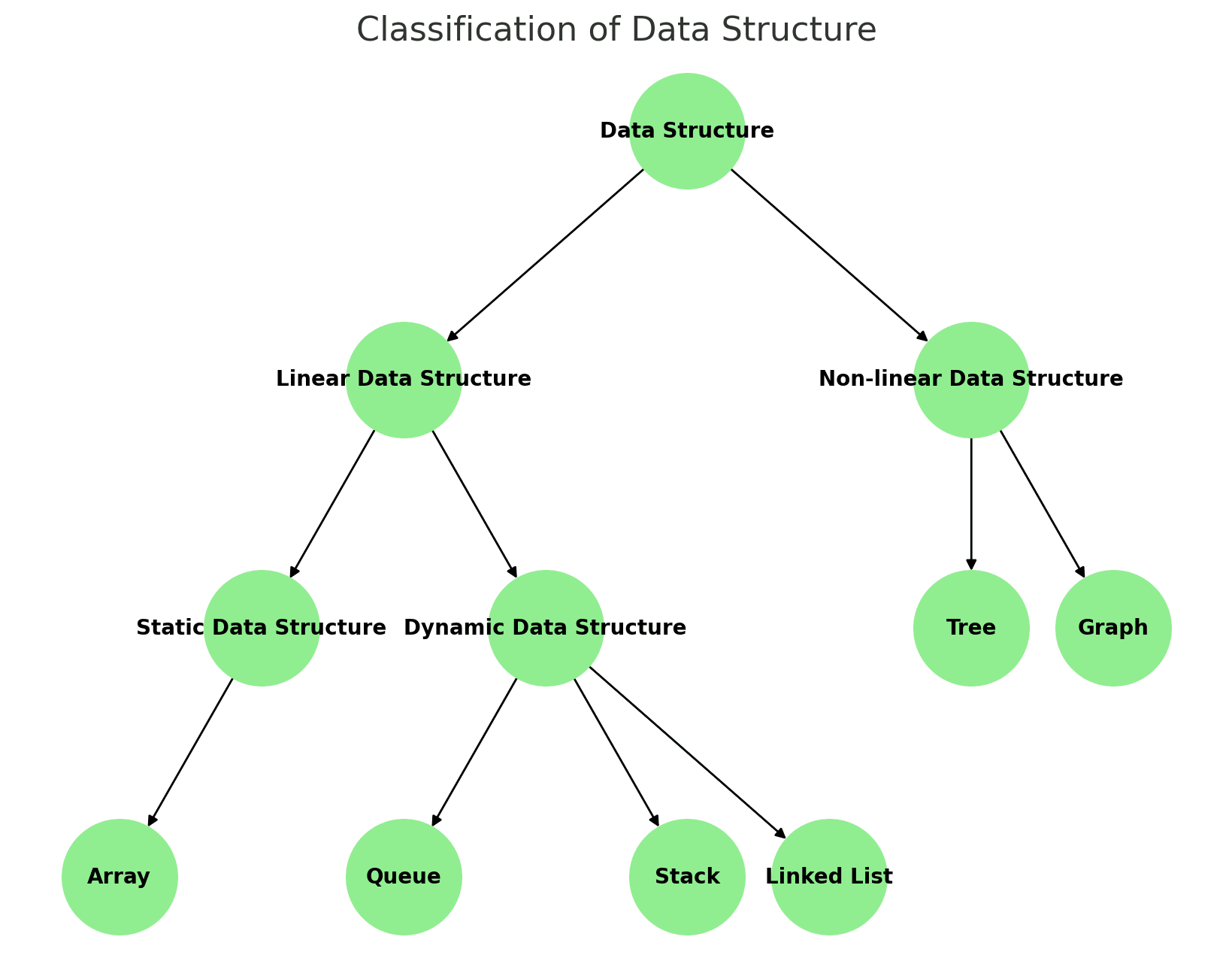
Introduction to Data Structure
Array
Linked List
Singly Linked List
A singly linked list is a linear collection of data items called nodes, where each node is divided into two parts.
- Data
- Link
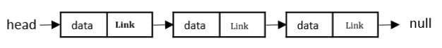
- The first node has a special name called HEAD.
- The data part stores the data item.
- The link part stores the address of the next node.
- The last node is called the tail node.
- The linked list starts with a special pointer called the HEAD pointer and terminates with a NULL pointer.
Singly Linked List
Singly linked list হলো একটি linear collection of data items, যেগুলোকে node বলা হয়। প্রতিটি node দুইটি অংশে বিভক্ত থাকে।
- Data
- Link
- প্রথম node-টির একটি বিশেষ নাম রয়েছে, যাকে HEAD বলা হয়।
- Data part-এ data item store করা হয়।
- Link part-এ পরবর্তী node-এর address store করা হয়।
- শেষ node-টিকে tail node বলা হয়।
- Linked list একটি বিশেষ pointer দিয়ে শুরু হয় যাকে HEAD pointer বলা হয় এবং এটি NULL pointer-এ শেষ হয়।
Declaration of Singly linked list:
struct node
{
  int data;
  struct node *next;
};
Doubly linked list is the linear collection of data item called node where each node has divided into three parts.
- previous
- data
- next
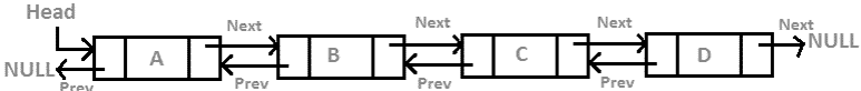
- Data part store data items.
- Next part store the address of next node
- previous part store the address of previous node.
- Doubly linked list start with special pointer called first pointer ending with last pointer.
- It allows us to perform traversing in both way “Forward & Backward”
Declaration of Doubly linked list:
struct node {
    int data;
    struct node *next;
    struct node *prev;
}
Circular linked list is the variation of singly and doubly linked list where first node point to last node and last node point to first node
It is used when we want traversing of data no. of time without reinitialized the start pointer as well as we can visit all the nodes from any nodes.
Types of Circular linked list:
- Circular singly Linked list
- Circular doubly linked list
A circular singly linked list is a type of linked list where the last node points to the first node instead of NULL.
This creates a circular structure, allowing traversal from any node continuously.
Key Point:
- Last node → points to first node
- No NULL pointer at the end
Declaration (C Language):
struct Node {
    int data;
    struct Node* next;
};

struct Node* head = NULL;
Diagram: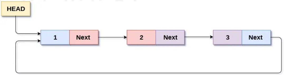
Circular singly linked list হলো এমন একটি linked list যেখানে last node প্রথম node-এর দিকে point করে, NULL নয়।
এভাবে list টি একটি circular structure তৈরি করে এবং যেকোনো node থেকে traversal চালানো যায়।
মূল বৈশিষ্ট্য:
- Last node → first node-এ point করে
- শেষে কোনো NULL থাকে না
Declaration (C Language):
struct Node {
    int data;
    struct Node* next;
};

struct Node* head = NULL;
Diagram:
A circular doubly linked list is a type of linked list where:
- The last node points to the first node
- The first node points back to the last node
This forms a circular structure in both directions (forward and backward).
Key Points:
- Each node has two pointers (prev and next)
- No NULL pointer at beginning or end
- Traversal is possible in both directions
Declaration (C Language):
struct Node {
    int data;
    struct Node* prev;
    struct Node* next;
};

struct Node* head = NULL;
Diagram: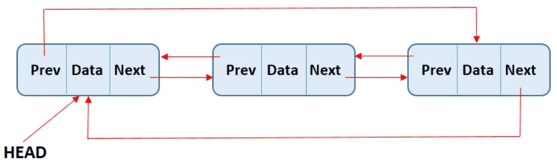
Circular doubly linked list হলো এমন একটি linked list যেখানে:
- Last node প্রথম node-এ point করে
- First node আবার last node-এ point করে
এটি forward এবং backward দুই দিকেই circular structure তৈরি করে।
মূল বৈশিষ্ট্য:
- প্রতিটি node-এ দুটি pointer (prev এবং next) থাকে
- শুরু বা শেষে কোনো NULL থাকে না
- দুই দিকেই traversal করা যায়
Declaration (C Language):
struct Node {
    int data;
    struct Node* prev;
    struct Node* next;
};

struct Node* head = NULL;
Diagram:
- Memory Use: Array uses contiguous memory with fixed size; Linked List uses non-contiguous memory and is dynamic.
- Access Speed: Array allows direct access (O(1)); Linked List requires sequential access (O(n)).
- Insertion/Deletion: Array is slow in middle/beginning; Linked List is faster if position is known.
- Memory Overhead: Array stores only data; Linked List stores data + pointer.
- Cache Performance: Array is faster due to better CPU cache usage; Linked List is slower.
- Flexibility: Array has fixed size; Linked List is flexible (can grow/shrink).
- Complexity: Array is simple; Linked List is complex due to pointer handling.
Array Representation: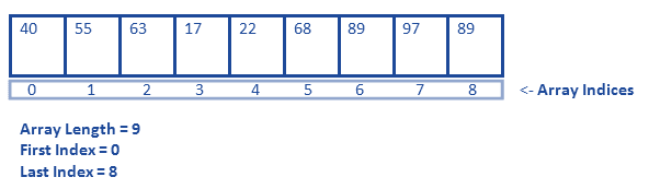
Linked List Representation: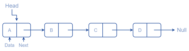
- Memory Use: Array contiguous memory ব্যবহার করে এবং fixed size; Linked List non-contiguous memory এবং dynamic।
- Access Speed: Array-এ direct access (O(1)); Linked List-এ sequential access (O(n))।
- Insertion/Deletion: Array-এ মাঝখানে ধীর; Linked List-এ position জানা থাকলে দ্রুত।
- Memory Overhead: Array শুধু data রাখে; Linked List data + pointer রাখে।
- Cache Performance: Array CPU cache-friendly তাই দ্রুত; Linked List ধীর।
- Flexibility: Array fixed size; Linked List সহজে grow/shrink করে।
- Complexity: Array সহজ; Linked List pointer ব্যবহারের কারণে জটিল।
Array Representation:
Linked List Representation:
Stack
When we define a stack as an Abstract Data Type (ADT), our primary focus is on the operations that can be performed on the stack, rather than how the stack is implemented internally.
The primary operations of a stack are as follows:
push(data): Adds a new element, data, onto the top of the stack.
pop(): Removes and returns the last element that was added to the stack (the topmost element).
top(): Retrieves the last inserted element from the stack without removing it, allowing you to peek at the top element.
size(): Returns the total number of elements currently in the stack.
isEmpty(): Checks if the stack is empty. Returns TRUE if the stack contains no elements, otherwise returns FALSE.
isFull(): Checks if the stack has reached its maximum capacity. Returns TRUE if the stack is full, otherwise returns FALSE.
Algorithm Insertion to Stack : PUSH operation
1. Checks if the stack is full.
2. If the stack is full, return "overflow" and exit.
3. If the stack is not full, increments top to point next
    empty space.
4. Adds data element to the stack location, where top
    is pointing.
5. Returns success.
pseudo-code of PUSH operation
PUSH(stack, data)
if stack is full:
    return "Overflow"  // Stack is full, cannot add more elements
else:
    top= top + 1  // Move to the next available position in the stack
    stack[top] = data    // Add the data element at the current top position
    return "Success"     // Data added successfully
Algorithm Insertion to Stack : POP operation
1. Checks if the stack is empty.
2. If the stack is empty, return underflow and exit.
3. If the stack is not empty, accesses the data element at
   which top is pointing.
4. Decreases the value of top by 1.
5. Returns success.
pseudo-code of POP operation
POP(stack)
if stack is empty:
    return "Underflow"  // Stack is empty, cannot remove elements
else:
   data = stack[top]   // Access the data element at the current top position
   top = top - 1  // Move the top pointer to the previous element
   return "Success"     // Data removed successfully
Infix expression: If operator is placed in between the operands then its called infix expression.
Infix Expression: <operand> <operator> <operand>
Example: A + B, A * B;
Prefix expression: If operator is placed before the operands then its called prefix expression.
Prefix Expression: <operator> <operand> <operand>
Example: +AB, *AB ;
Postfix expression: If operator is placed after the operands then its called postfix expression.
Postfix Expression: <operand> <operand> <operator>
Example: AB+, AB* ;
(i) (A + B) * (B * D)
(ii) (a+b)*c
(iii)a/b+c/d
(iv)(a+b*d)*(b-c)
(i) (A + B) * (B * D)
= (AB+) * (BD*)
= AB+ BD* *
(ii) (a+b)*c
= (ab+) * c
= ab+c*
(iii) a/b+c/d
= (ab/) + (cd/)
= ab/cd/+
(iv) (a+b*d)*(b-c)
=(a+(bd*))*(bc-)
=(abd*+)*(bc-)
=abd*+bc-*
(i) (A + B) * (B * D)
(ii) (a+b)*c
(iii)a/b+c/d
(iv)(a+b*d)*(b-c)
(v) ((a+b)*c)-d
(i) (A + B) * (B * D)
= (+AB) * (*BD)
= *+AB *BD
(ii) (a+b)*c
= (+ab) * c
= *+abc
(iii) a/b+c/d
= (/ab) + (/cd)
= +/ab/cd
(iv) (a+b*d)*(b-c)
=(a+(*bd))*(-bc)
=(+a*bd)*(-bc)
=*+a*bd-bc
(v) ((a+b)*c)-d
=((+ab)*c)-d
=(*+abc)-d
= – * + abcd
(i) ABD*+BC-*
(ii) ab+cd+*
(i) ABD*+BC-*
= A (B*D)+BC-*
= (A+(B*D))BC-*
=(A+(B*D))(B-C)*
=(A+(B*D))*(B-C)
(ii) ab+cd+*
= (a+b)cd+*
= (a+b) (c+d)*
= (a+b) * (c+d)
(i) -*+abcd
(ii)/+A*BD-BC
(iii)+/ab/cd
(i) -*+abcd
= -*(a+b)cd
= -((a+b)*c)d
=((a+b)*c)-d
(ii) /+A*BD-BC
= /+A(B*D)-BC
= /(A+(B*D))-BC
= /(A+(B*D))(B-C)
= (A+(B*D))/(B-C)
(iii)+/ab/cd
=+(a/b)/cd
=+(a/b)(c/d)
=(a/b)+(c/d)
Below is the algorithm to convert an infix expression to postfix notation:
- Initialize:
- Push
"("onto the Stack. - Add
")"to the end of the expressionX.
- Push
- Scan Expression
Xfrom left to right:- Repeat Steps 3 to 6 for each element of
Xuntil the Stack is empty.
- Repeat Steps 3 to 6 for each element of
- If the character is an operand:
- Add the operand directly to
Y.
- Add the operand directly to
- If the character is a left parenthesis
"(":- Push
"("onto the Stack.
- Push
- If the character is an operator:
- Repeatedly pop operators from the Stack and add them to
Ywhile the operator at the top of the Stack has equal or higher precedence than the current operator. - Push the current operator onto the Stack.
- Repeatedly pop operators from the Stack and add them to
- If the character is a right parenthesis
")":- Repeatedly pop operators from the Stack and add them to
Yuntil a left parenthesis"("is encountered. - Remove the left parenthesis from the Stack.
- Repeatedly pop operators from the Stack and add them to
- End of Expression:
- Once the entire expression is processed, the final postfix expression
Ywill be available in the output.
- Once the entire expression is processed, the final postfix expression
Example
Infix to Postfix Conversion Stack Table
A+B/C*(D+E)-F
Adding “)” at the end of expression =A+B/C*(D+E)-F)
| Scan | Stack | Postfix Expression |
|---|---|---|
| ( | ||
| A | ( | A |
| + | (+ | A |
| B | (+ | A B |
| / | (+ / | A B |
| C | (+ / | A B C |
| * | (+ * | A B C / |
| ( | (+ * ( | A B C / |
| D | (+ * ( | A B C / D |
| + | (+ * ( + | A B C / D |
| E | (+ * ( + | A B C / D E |
| ) | (+ * | A B C / D E + |
| – | (- | A B C / D E + * |
| F | (- | A B C / D E + * + F |
| ) | A B C / D E + * + F – |
Postfix expression: A B C / D E + * + F –
Below is the algorithm to evaluate a postfix expression:
- Initialize:
- Create an empty stack.
- Scan the postfix expression from left to right:
- Repeat the following steps for each symbol in the expression.
- If the symbol is an operand (a number or a variable):
- Push the operand’s value onto the stack.
- If the symbol is an operator (+, -, *, /, ^, etc.):
- Pop the top two operands from the stack.
- Let the first popped operand be
operand1and the second popped operand beoperand2. - Perform the operation:
operand2 operator operand1. - Push the result of this operation back onto the stack.
- After scanning the entire expression:
- The final result of the evaluation will be the only value remaining on the stack.
- Pop this value and return it as the result of the expression.
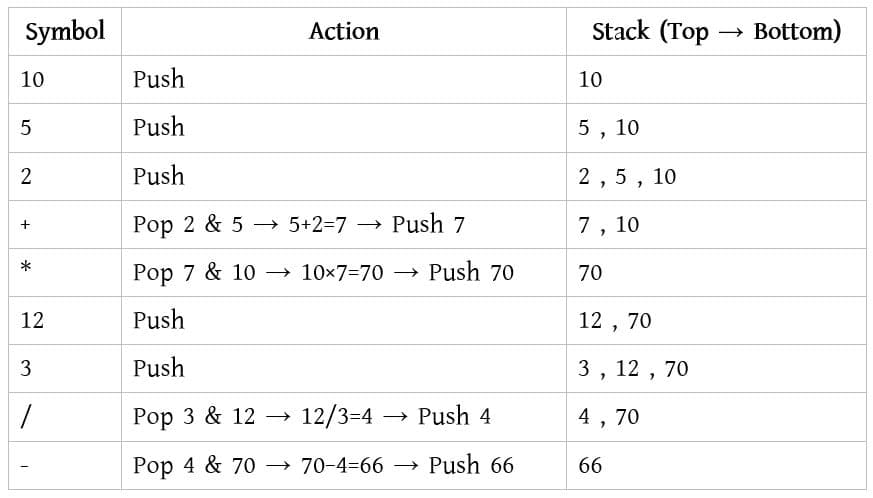
Example: P = 12 7 3 – / 2 +
✔ 12 → Push onto stack → Stack: [12]
✔ 7 → Push onto stack → Stack: [12, 7]
✔ 3 → Push onto stack → Stack: [12, 7, 3]
✔ – → Pop 7 and 3, perform 7 – 3 = 4 → Push 4 → Stack: [12, 4]
✔ / → Pop 12 and 4, perform 12 / 4 = 3 → Push 3 → Stack: [3]
✔ 2 → Push onto stack → Stack: [3, 2]
✔ + → Pop 3 and 2, perform 3 + 2 = 5 → Push 5 → Stack: [5]
The evaluated value of the expression is: P = 5
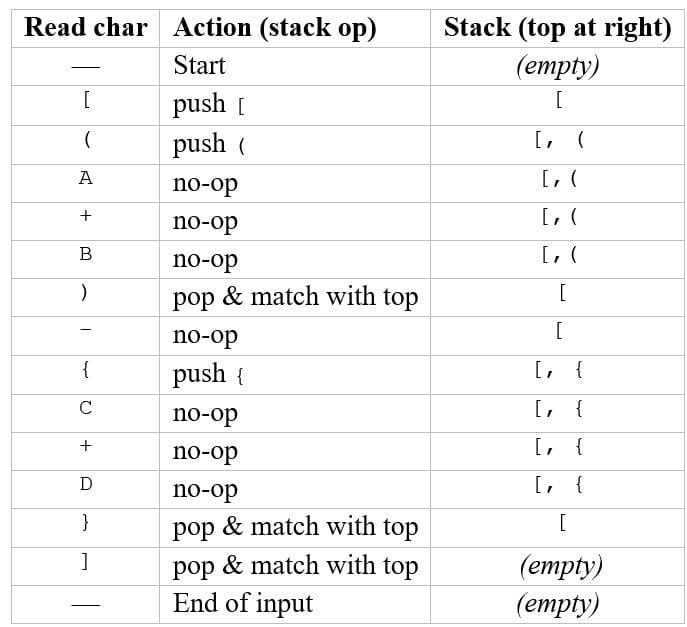
[(A+B)-{C+D}]
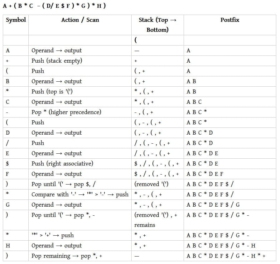
A + ( B * C − ( D / E $ F ) * G) * H
10 5 2 + * 12 3 / -
Queue
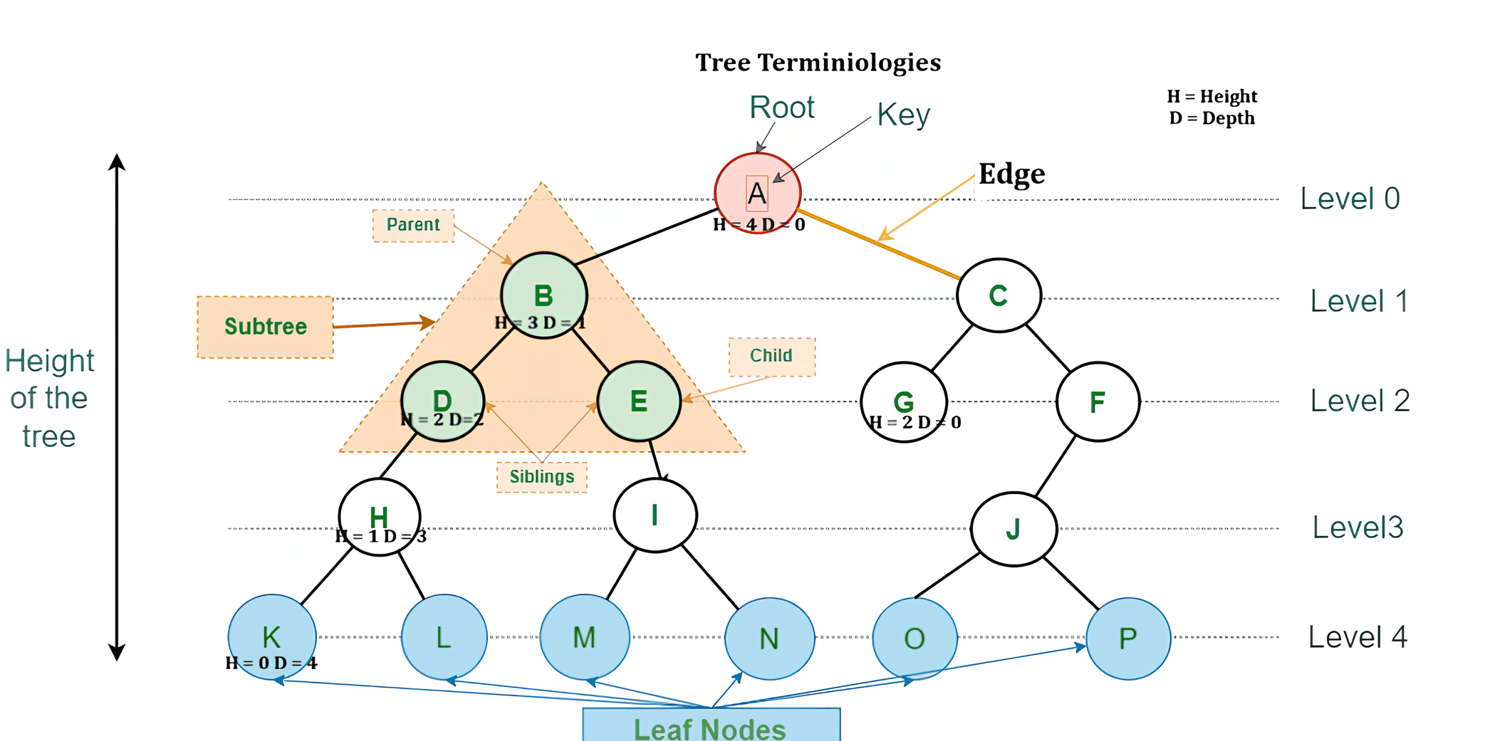
Tree Data Structure
8
/ \
2 10
\
26
\
78
\
102
\
115
5
/ \
4 10
\
90
/ \
60 98
/
50
\
55
Mathematics
/ \
Geography Physics
/ \ / \
Chemistry Geology Meteorology Zoology
/
Psychology
Inorder: D B E A F C
Preorder: A B D E C F
Construction of Binary Tree from Preorder and Inorder Traversal (Step by Step)
Given
Inorder: D B E A F C
Preorder: A B D E C F
Rule
1) In Preorder, the first element is always the Root.
2) In Inorder, elements left of Root belong to Left Subtree, and elements right of Root belong to Right Subtree.
Step 1: Find Root
Preorder = A B D E C F → Root = A
Now locate A in Inorder: D B E A F C
Left(Inorder) = D B E
Right(Inorder) = F C
Step 2: Build Left Subtree of A
Left(Inorder) = D B E (3 nodes) → so next 3 nodes in Preorder after A belong to left subtree.
Preorder after A = B D E … → Left(Preorder) = B D E
Now for Left subtree:
Preorder = B D E → Root = B
Find B in Inorder: D B E
Left of B (Inorder) = D
Right of B (Inorder) = E
So B’s left child = D, B’s right child = E
Step 3: Build Right Subtree of A
Right(Inorder) = F C (2 nodes) → remaining Preorder nodes belong to right subtree.
Remaining Preorder = C F → Right(Preorder) = C F
Now for Right subtree:
Preorder = C F → Root = C
Find C in Inorder: F C
Left of C (Inorder) = F
Right of C (Inorder) = (none)
So C’s left child = F, C has no right child.
Final Constructed Binary Tree
            A
           / \
          B   C
/ \ /
D E FConstruction of Binary Tree and Finding Height (Step by Step)
Given
Postorder Traversal: 8, 9, 6, 7, 4, 5, 2, 3, 1
Inorder Traversal: 8, 3, 9, 4, 7, 2, 5, 1, 6
Rule Used
1) In Postorder, the last element is always the Root.
2) In Inorder, elements to the left of the root belong to the left subtree and elements to the right belong to the right subtree.
Step 1: Identify Root
Postorder last element = 1 → Root of the tree is 1.
Inorder split at 1:
Left(Inorder) = 8, 3, 9, 4, 7, 2, 5
Right(Inorder) = 6
Step 2: Construct Right Subtree
Right(Inorder) has only one node → Right child of 1 is 6.
Step 3: Construct Left Subtree
Remaining Postorder (before 1) = 8, 9, 6, 7, 4, 5, 2, 3
Last element here = 3 → Root of left subtree.
Inorder split at 3:
Left of 3 = 8
Right of 3 = 9, 4, 7, 2, 5
Continuing this process recursively, the left subtree is constructed.
Final Binary Tree Structure
            1
           / \
          3   6
         / \
        8   2
           / \
          4   5
         / \
        9   7
Step 4: Find Height of the Tree
Height of a binary tree is the number of edges on the longest path from root to a leaf.
Longest path here is:
1 → 3 → 2 → 4 → 9
This path has 4 edges.
Final Answer
The height of the given binary tree is 4.
            /
          /   \
        -       +
       / \     / \
      a   b   *   e
             / \
            c   d
                 +
               /   \
             ^       -
           /   \    / \
         +      3  *   y
        / \        / \
      *   *      2   x
     / \ / \
    3  x 4  z
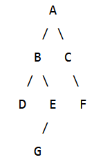 1) Write the Inorder Traversal of the above binary tree.
2) Write the Preorder Traversal of the above binary tree.
3) Write the Postorder Traversal of the above binary tree.
Inorder Traversal:
D B G E A C F
Preorder Traversal:
A B D E G C F
Postorder Traversal:
D G E B F C A
Heap Data Structure
Graph Data Structure
Types of Graphs in Data Structure and Algorithms
A graph can be classified into different types based on properties such as weight, direction of edges, and connectivity.
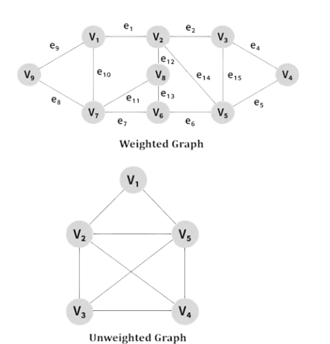
Based on Weight
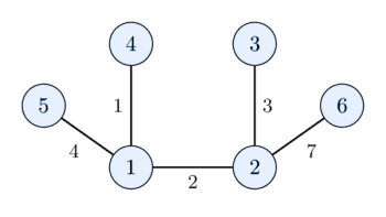
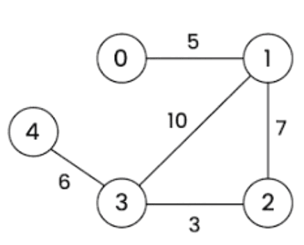
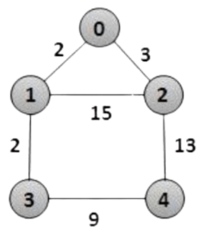
- Weighted Graph: A graph in which each edge is assigned a weight representing cost, distance, or time.
- Unweighted Graph: A graph in which all edges are treated equally and do not have any associated weight.
Based on Edge Direction
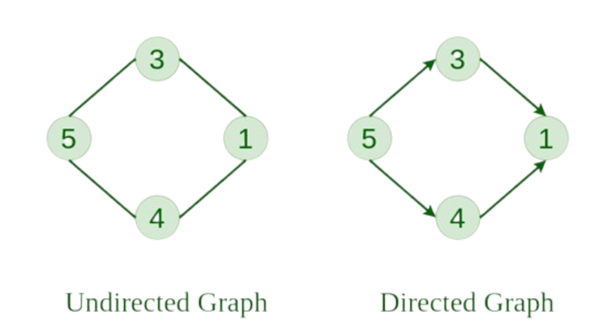
- Undirected Graph: A graph in which edges have no direction. Each edge represents an unordered pair of vertices.
- Directed Graph: A graph in which edges have a direction. Each edge represents an ordered pair of vertices.
Data Structure এবং Algorithms-এ Graph-এর ধরন
Graph-কে বিভিন্ন বৈশিষ্ট্যের উপর ভিত্তি করে শ্রেণিবদ্ধ করা যায়, যেমন weight, edge-এর direction এবং connectivity।
Weight-এর ভিত্তিতে
- Weighted Graph: Weighted Graph-এ প্রতিটি edge-এর সাথে একটি weight থাকে, যা cost, distance বা time নির্দেশ করে।
- Unweighted Graph: Unweighted Graph-এ সব edge সমানভাবে বিবেচিত হয় এবং কোনো weight থাকে না।
Edge Direction-এর ভিত্তিতে
- Undirected Graph: Undirected Graph-এ edge-এর কোনো direction থাকে না। এখানে vertex-গুলো unordered pair হিসেবে যুক্ত থাকে।
- Directed Graph: Directed Graph-এ edge-এর নির্দিষ্ট direction থাকে এবং vertex-গুলো ordered pair হিসেবে যুক্ত হয়।
Graph Representation
Graphs are commonly represented in two ways:
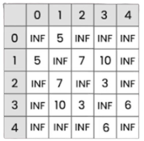
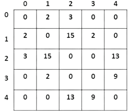
1. Adjacency Matrix
An Adjacency Matrix is a 2D array of size V × V, where V is the number of vertices. Each row and column represent a vertex.
If the value of a[i][j] is 1, it indicates that there is an edge between vertex i and vertex j; otherwise, the value is 0.
In an undirected graph, the adjacency matrix is symmetric about the diagonal because if (i, j) is an edge, then (j, i) is also an edge.
Advantage: Edge lookup is very fast.
Disadvantage: Requires large memory space (V × V).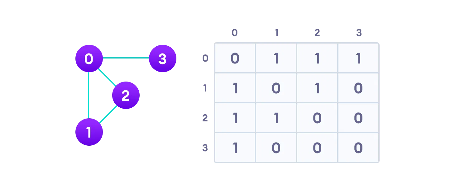
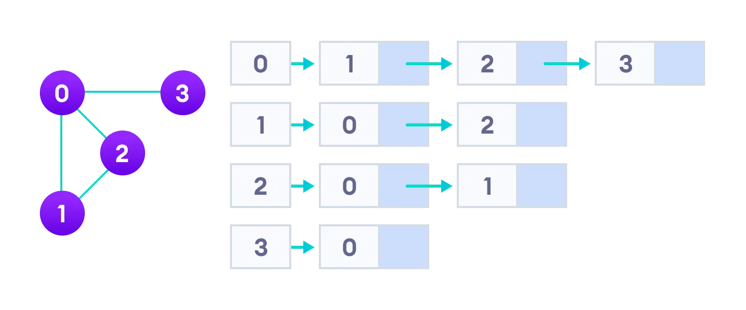
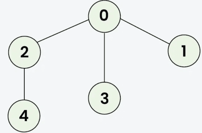
2. Adjacency List
An Adjacency List represents a graph as an array of linked lists. Each index of the array represents a vertex, and each linked list stores the vertices connected to that vertex.
This representation stores only existing edges, making it more space-efficient.
Advantage: Efficient in terms of storage, especially for large graphs.
Graph Representation
Graph সাধারণত দুইভাবে represent করা হয়:
1. Adjacency Matrix
Adjacency Matrix হলো V × V আকারের একটি 2D array, যেখানে V হলো vertex-এর সংখ্যা। প্রতিটি row এবং column একটি vertex নির্দেশ করে।
যদি a[i][j] এর মান 1 হয়, তাহলে vertex i এবং vertex j-এর মধ্যে একটি edge আছে; না হলে মান 0 হয়।
Undirected graph-এর ক্ষেত্রে adjacency matrix diagonal-এর চারপাশে symmetric হয়, কারণ (i, j) edge থাকলে (j, i) edge-ও থাকবে।
Advantage: Edge আছে কিনা তা খুব দ্রুত জানা যায়।
Disadvantage: V × V space প্রয়োজন হয়, ফলে memory বেশি লাগে।
2. Adjacency List
Adjacency List-এ graph-কে একটি array of linked lists হিসেবে represent করা হয়। Array-এর প্রতিটি index একটি vertex নির্দেশ করে এবং linked list-এ ঐ vertex-এর সাথে যুক্ত অন্য vertex-গুলো থাকে।
এই পদ্ধতিতে শুধুমাত্র existing edge গুলো store করা হয়, তাই memory কম লাগে।
Advantage: Large graph-এর জন্য খুবই space-efficient।
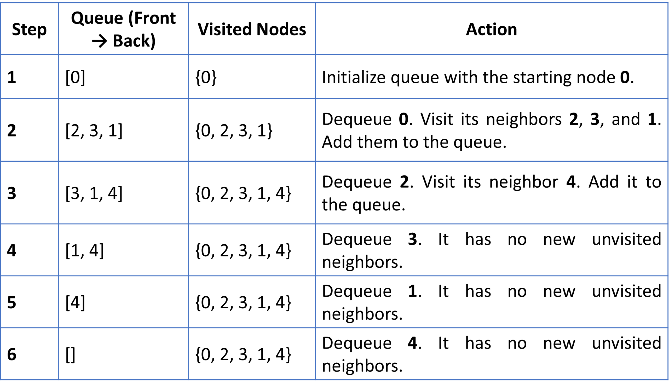
BFS Traversal:
👉 0, 2, 3, 1, 4
To perform a Breadth-First Search (BFS) on the provided graph, we explore the nodes level by level, starting from a source node (typically 0).
BFS uses a Queue (First-In-First-Out) to keep track of which nodes to visit next and a Visited list to ensure we don’t process the same node twice.
BFS Step by Step Execution:
Final BFS Traversal Order
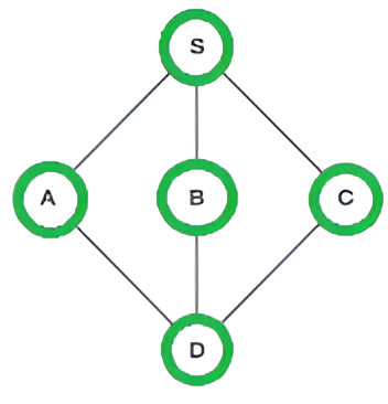
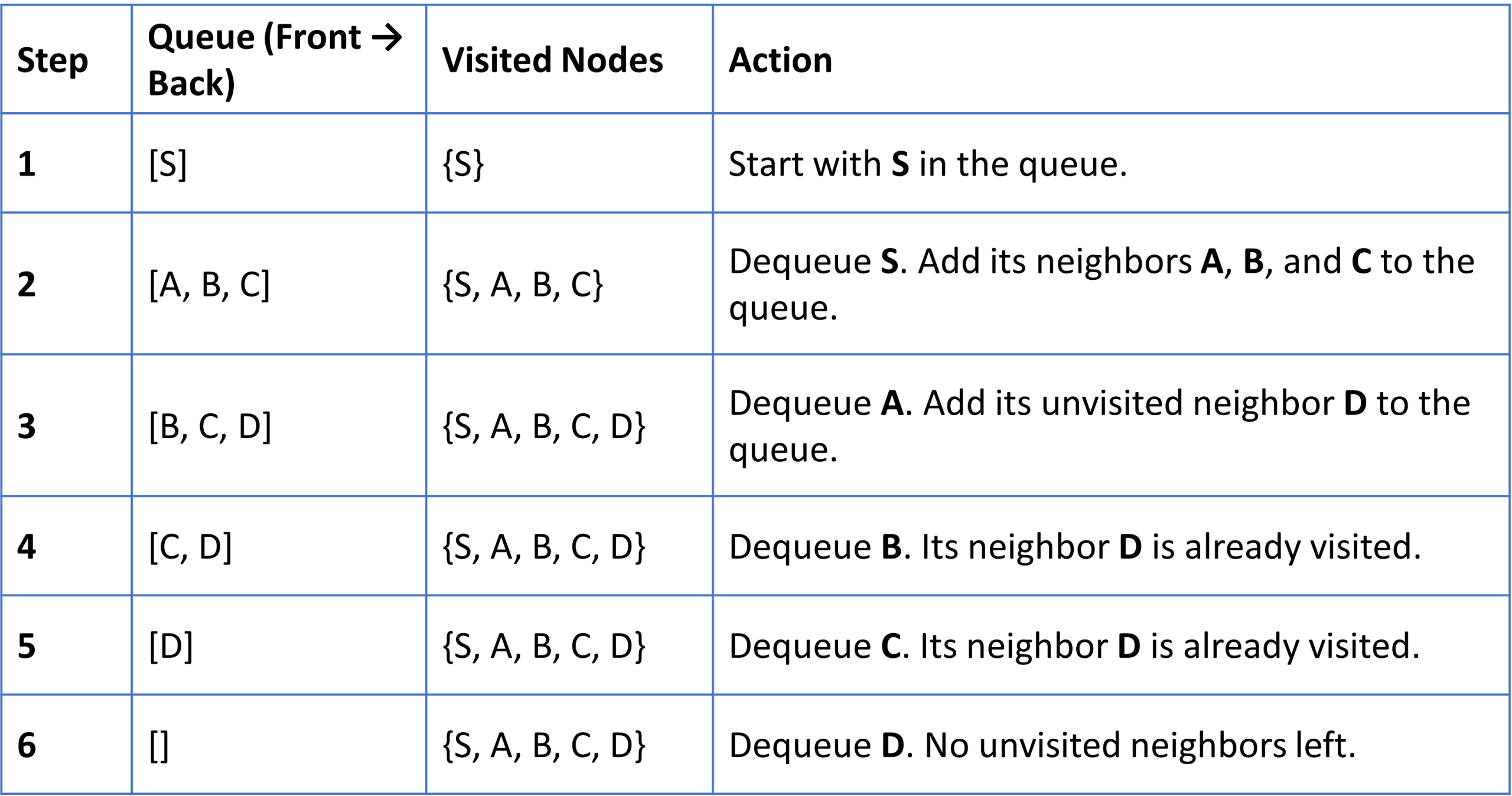
The order of exploration is: S → A → B → C → D
To perform a Breadth-First Search (BFS) on this graph, we start from a source node (typically S) and explore all of its immediate neighbors before moving to the next level of depth.
BFS uses a Queue (First-In, First-Out) and a Visited set to track progress.
BFS Step-by-Step Execution
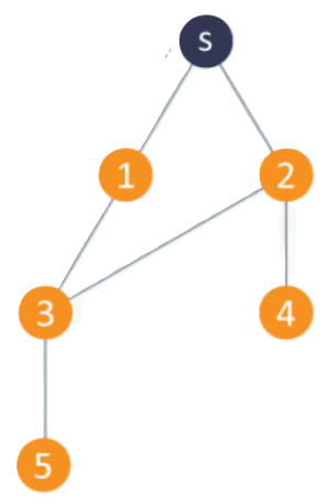
To perform a Depth-First Search (DFS) on this graph starting from node S, we follow one branch as deep as possible before backtracking to explore other branches.
DFS typically uses a Stack (Last-In, First-Out) or recursion. When multiple neighbors are available, it is standard practice to visit them in numerical order.
DFS Step-by-Step Execution: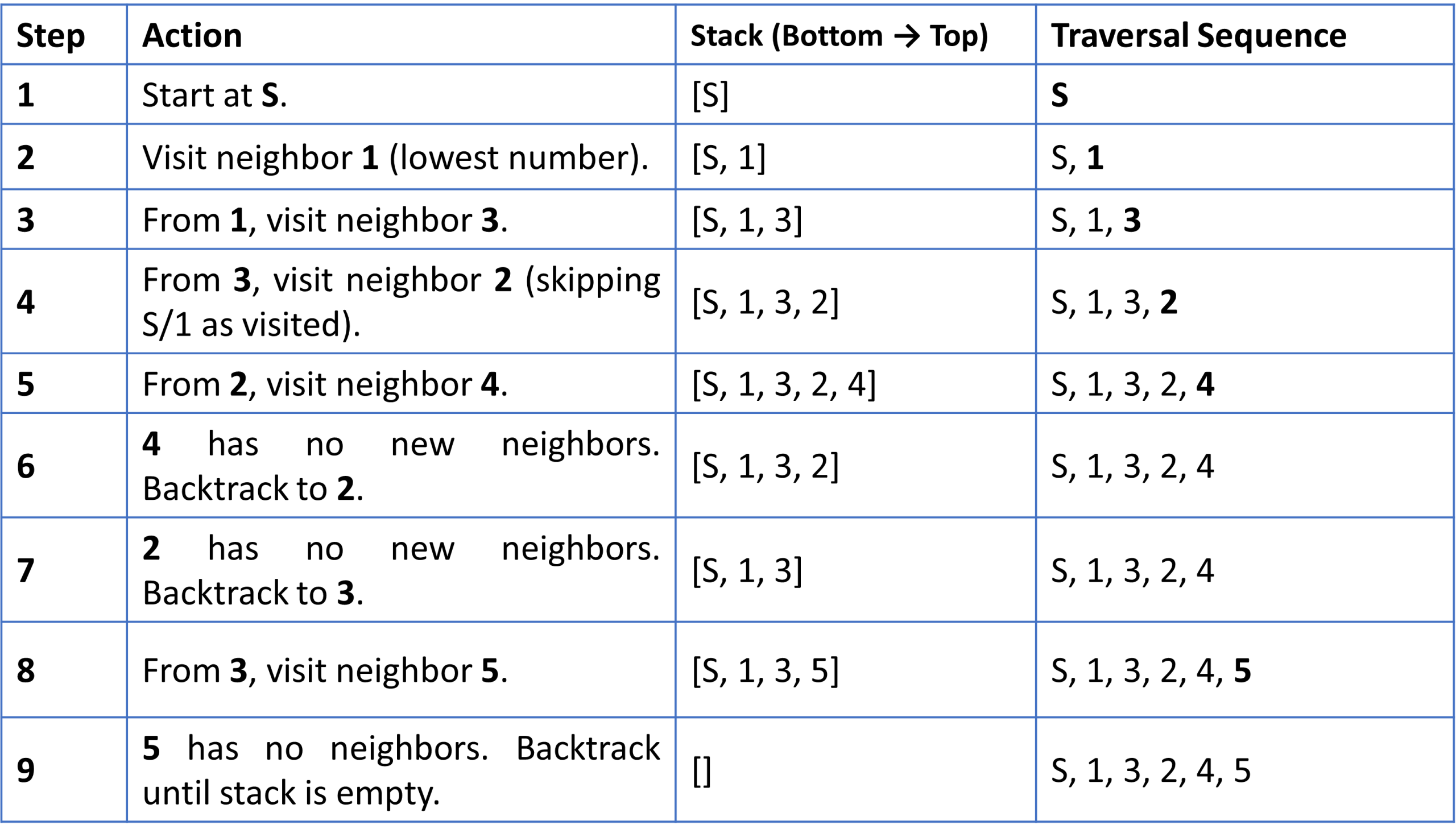
Example:
- Civil Network Planning
- Computer Network Routing Protocol
- Cluster Analysis
Example: