Introduction to Algorithm
Searching Algorithm
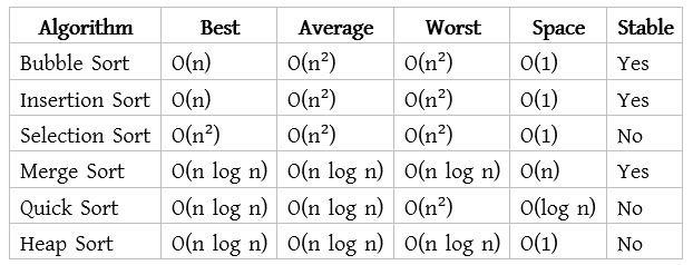
Sorting Algorithm
bubbleSort(array)
for i ← 1 to sizeOfArray − 1 do
    for j ← 1 to sizeOfArray − 1 − i do
        if array[j] > array[j + 1] then
           swap array[j] and array[j + 1]
        end if
    end for
end for
end bubbleSort
Bubble Sort (Ascending) — Step-by-step Iterations
Initial List: [30, 25, 62, 45, 7, 10]
Pass 1 (i = 1)
1) Compare 30 and 25 → swap → [25, 30, 62, 45, 7, 10]
2) Compare 30 and 62 → no swap → [25, 30, 62, 45, 7, 10]
3) Compare 62 and 45 → swap → [25, 30, 45, 62, 7, 10]
4) Compare 62 and 7 → swap → [25, 30, 45, 7, 62, 10]
5) Compare 62 and 10 → swap → [25, 30, 45, 7, 10, 62]
End of Pass 1: [25, 30, 45, 7, 10, 62]
Pass 2 (i = 2)
1) Compare 25 and 30 → no swap → [25, 30, 45, 7, 10, 62]
2) Compare 30 and 45 → no swap → [25, 30, 45, 7, 10, 62]
3) Compare 45 and 7 → swap → [25, 30, 7, 45, 10, 62]
4) Compare 45 and 10 → swap → [25, 30, 7, 10, 45, 62]
End of Pass 2: [25, 30, 7, 10, 45, 62]
Pass 3 (i = 3)
1) Compare 25 and 30 → no swap → [25, 30, 7, 10, 45, 62]
2) Compare 30 and 7 → swap → [25, 7, 30, 10, 45, 62]
3) Compare 30 and 10 → swap → [25, 7, 10, 30, 45, 62]
End of Pass 3: [25, 7, 10, 30, 45, 62]
Pass 4 (i = 4)
1) Compare 25 and 7 → swap → [7, 25, 10, 30, 45, 62]
2) Compare 25 and 10 → swap → [7, 10, 25, 30, 45, 62]
End of Pass 4: [7, 10, 25, 30, 45, 62]
Pass 5 (i = 5)
1) Compare 7 and 10 → no swap → [7, 10, 25, 30, 45, 62]
End of Pass 5: [7, 10, 25, 30, 45, 62]
Note: No swaps happened, so the list is already sorted (early stop).
Final Sorted List (Ascending): [7, 10, 25, 30, 45, 62]
Algorithm (Steps)
1) Start from the first element of the array.
2) Assume the first element is the minimum element.
3) Compare this minimum element with the remaining elements of the array.
4) If a smaller element is found, update the minimum element.
5) Swap the minimum element with the first element of the unsorted part.
6) Move the boundary of the sorted part one position forward.
7) Repeat the above steps until the entire array is sorted.
selectionSort(array)
  for i ← 1 to sizeOfArray − 1
    minIndex ← i
    for j ← i + 1 to sizeOfArray
      if array[j] < array[minIndex]
        minIndex ← j
    end for
    if minIndex ≠ i
      swap array[i] and array[minIndex]
  end for
end selectionSort
[urcr_restrict]
Insertion Sort — Step-by-step Execution
Initial Array: [30, 25, 62, 45, 7, 10]
Pass 1 (i = 2, key = 25)
Compare 25 with 30 → shift 30 to the right
Insert 25 at position 1
Array after Pass 1: [25, 30, 62, 45, 7, 10]
Pass 2 (i = 3, key = 62)
Compare 62 with 30 → no shift required
Array after Pass 2: [25, 30, 62, 45, 7, 10]
Pass 3 (i = 4, key = 45)
Compare 45 with 62 → shift 62 to the right
Compare 45 with 30 → stop shifting
Insert 45 in correct position
Array after Pass 3: [25, 30, 45, 62, 7, 10]
Pass 4 (i = 5, key = 7)
Compare 7 with 62 → shift 62 to the right
Compare 7 with 45 → shift 45 to the right
Compare 7 with 30 → shift 30 to the right
Compare 7 with 25 → shift 25 to the right
Insert 7 at the beginning
Array after Pass 4: [7, 25, 30, 45, 62, 10]
Pass 5 (i = 6, key = 10)
Compare 10 with 62 → shift 62 to the right
Compare 10 with 45 → shift 45 to the right
Compare 10 with 30 → shift 30 to the right
Compare 10 with 25 → shift 25 to the right
Compare 10 with 7 → stop shifting
Insert 10 in correct position
Array after Pass 5: [7, 10, 25, 30, 45, 62]
Final Sorted Array (Ascending Order): [7, 10, 25, 30, 45, 62][/urcr_restrict]
Algorithm (Steps)
1) Start from the first element of the array.
2) Find the smallest element in the unsorted part of the array.
3) Swap it with the first unsorted element.
4) Move the boundary of sorted and unsorted part one step forward.
5) Repeat the process for the remaining elements.
6) Continue until the entire array is sorted.
selectionSort(array, n)
  for i ← 0 to n − 2
    minIndex ← i
    for j ← i + 1 to n − 1
      if array[j] < array[minIndex]
        minIndex ← j
    swap array[i] and array[minIndex]
end selectionSort
[urcr_restrict]
Selection Sort — Step-by-step Example
Given Array: [30, 25, 62, 45, 7, 10]
Pass 1 (i = 1)
Assume minimum = 30
Compare 30 with 25 → new minimum = 25
Compare 25 with 62 → no change
Compare 25 with 45 → no change
Compare 25 with 7 → new minimum = 7
Compare 7 with 10 → no change
Swap 30 and 7
Array after Pass 1: [7, 25, 62, 45, 30, 10]
Pass 2 (i = 2)
Assume minimum = 25
Compare 25 with 62 → no change
Compare 25 with 45 → no change
Compare 25 with 30 → no change
Compare 25 with 10 → new minimum = 10
Swap 25 and 10
Array after Pass 2: [7, 10, 62, 45, 30, 25]
Pass 3 (i = 3)
Assume minimum = 62
Compare 62 with 45 → new minimum = 45
Compare 45 with 30 → new minimum = 30
Compare 30 with 25 → new minimum = 25
Swap 62 and 25
Array after Pass 3: [7, 10, 25, 45, 30, 62]
Pass 4 (i = 4)
Assume minimum = 45
Compare 45 with 30 → new minimum = 30
Compare 30 with 62 → no change
Swap 45 and 30
Array after Pass 4: [7, 10, 25, 30, 45, 62]
Pass 5 (i = 5)
Assume minimum = 45
Compare 45 with 62 → no change
No swap needed
Array after Pass 5: [7, 10, 25, 30, 45, 62]
Final Sorted Array (Ascending Order): [7, 10, 25, 30, 45, 62][/urcr_restrict]
[urcr_restrict]
Algorithm (Steps)
1) Divide the given array into two halves.
2) Recursively apply Merge Sort on the left half.
3) Recursively apply Merge Sort on the right half.
4) Merge the two sorted halves into a single sorted array.
5) Repeat the process until the entire array is sorted.
mergeSort(array, left, right)
  if left < right
    mid ← (left + right) / 2
    mergeSort(array, left, mid)
    mergeSort(array, mid + 1, right)
    merge(array, left, mid, right)
end mergeSort

merge(array, left, mid, right)
  n1 ← mid − left + 1
  n2 ← right − mid

  create array L[1..n1] and R[1..n2]

  for i ← 1 to n1
    L[i] ← array[left + i − 1]

  for j ← 1 to n2
    R[j] ← array[mid + j]

  i ← 1, j ← 1, k ← left

  while i ≤ n1 and j ≤ n2
    if L[i] ≤ R[j]
      array[k] ← L[i]
      i ← i + 1
    else
      array[k] ← R[j]
      j ← j + 1
    k ← k + 1

  while i ≤ n1
    array[k] ← L[i]
    i ← i + 1
    k ← k + 1

  while j ≤ n2
    array[k] ← R[j]
    j ← j + 1
    k ← k + 1
end merge
[/urcr_restrict]
Merge Sort — Step-by-step Example (Ascending)
Given Array: [30, 25, 62, 45, 7, 10]
Step 1: Divide (Split) the array
Split into two halves:
Left = [30, 25, 62]
Right = [45, 7, 10]
Step 2: Divide the Left half
Left = [30, 25, 62] → Split into:
L1 = [30, 25]
L2 = [62]
Step 3: Divide L1 further
L1 = [30, 25] → Split into:
[30] and [25]
Step 4: Merge (Sort) [30] and [25]
Merge → [25, 30]
Step 5: Merge [25, 30] and [62]
Merge → [25, 30, 62]
Sorted Left Half: [25, 30, 62]
Step 6: Divide the Right half
Right = [45, 7, 10] → Split into:
R1 = [45, 7]
R2 = [10]
Step 7: Divide R1 further
R1 = [45, 7] → Split into:
[45] and [7]
Step 8: Merge (Sort) [45] and [7]
Merge → [7, 45]
Step 9: Merge [7, 45] and [10]
Merge → [7, 10, 45]
Sorted Right Half: [7, 10, 45]
Step 10: Final Merge of two sorted halves
Merge [25, 30, 62] and [7, 10, 45]:
Result → [7, 10, 25, 30, 45, 62]
Final Sorted Array (Ascending Order): [7, 10, 25, 30, 45, 62]
<
Algorithm (Steps)
1) Choose a pivot element from the array.
2) Rearrange the array so that elements smaller than the pivot are on the left and larger elements are on the right.
3) Place the pivot in its correct position.
4) Recursively apply Quick Sort on the left subarray.
5) Recursively apply Quick Sort on the right subarray.
6) Repeat the process until the entire array is sorted.
quickSort(array, low, high)
  if low < high
    pivotIndex ← partition(array, low, high)
    quickSort(array, low, pivotIndex − 1)
    quickSort(array, pivotIndex + 1, high)
end quickSort

partition(array, low, high)
  pivot ← array[high]
  i ← low − 1
  for j ← low to high − 1
    if array[j] < pivot
      i ← i + 1
      swap array[i] and array[j]
  swap array[i + 1] and array[high]
  return i + 1
Given list:
41, 25, 87, 57, 80, 79, 19, 36, 42, 7
Quick Sort idea:
Choose a pivot, then place smaller elements on the left and larger elements on the right. Repeat the same process for each sub-list.
Here I use the first element as pivot in each step.
Step 1: Sort the full list
List: 41, 25, 87, 57, 80, 79, 19, 36, 42, 7
Pivot = 41
Elements smaller than 41: 25, 19, 36, 7
Elements greater than 41: 87, 57, 80, 79, 42
So now:
25, 19, 36, 7 | 41 | 87, 57, 80, 79, 42
Step 2: Sort left sub-list
Sub-list: 25, 19, 36, 7
Pivot = 25
Elements smaller than 25: 19, 7
Elements greater than 25: 36
So:
19, 7 | 25 | 36
Step 3: Sort the left part of that sub-list
Sub-list: 19, 7
Pivot = 19
Elements smaller than 19: 7
Elements greater than 19: none
So:
7 | 19
Now the full left side becomes:
7, 19, 25, 36
Step 4: Sort right sub-list of 41
Sub-list: 87, 57, 80, 79, 42
Pivot = 87
Elements smaller than 87: 57, 80, 79, 42
Elements greater than 87: none
So:
57, 80, 79, 42 | 87
Step 5: Sort 57, 80, 79, 42
Pivot = 57
Elements smaller than 57: 42
Elements greater than 57: 80, 79
So:
42 | 57 | 80, 79
Step 6: Sort 80, 79
Pivot = 80
Elements smaller than 80: 79
Elements greater than 80: none
So:
79 | 80
Now the full right side becomes:
42, 57, 79, 80, 87
Step 7: Combine everything
Left side: 7, 19, 25, 36
Pivot: 41
Right side: 42, 57, 79, 80, 87
Final sorted list:
7, 19, 25, 36, 41, 42, 57, 79, 80, 87
Given Array: 170, 45, 75, 90, 802, 24, 2, 66
Radix Sort sorts numbers digit by digit (from Least Significant Digit – LSD to Most Significant Digit).
Step 1: Sort by Unit Digit (1’s place)
- 170 → 0
- 45 → 5
- 75 → 5
- 90 → 0
- 802 → 2
- 24 → 4
- 2 → 2
- 66 → 6
After sorting: 170, 90, 802, 2, 24, 45, 75, 66
Step 2: Sort by Tens Digit (10’s place)
- 170 → 7
- 90 → 9
- 802 → 0
- 2 → 0
- 24 → 2
- 45 → 4
- 75 → 7
- 66 → 6
After sorting: 802, 2, 24, 45, 66, 170, 75, 90
Step 3: Sort by Hundreds Digit (100’s place)
- 802 → 8
- 2 → 0
- 24 → 0
- 45 → 0
- 66 → 0
- 170 → 1
- 75 → 0
- 90 → 0
After sorting (Final Output): 2, 24, 45, 66, 75, 90, 170, 802 ✅
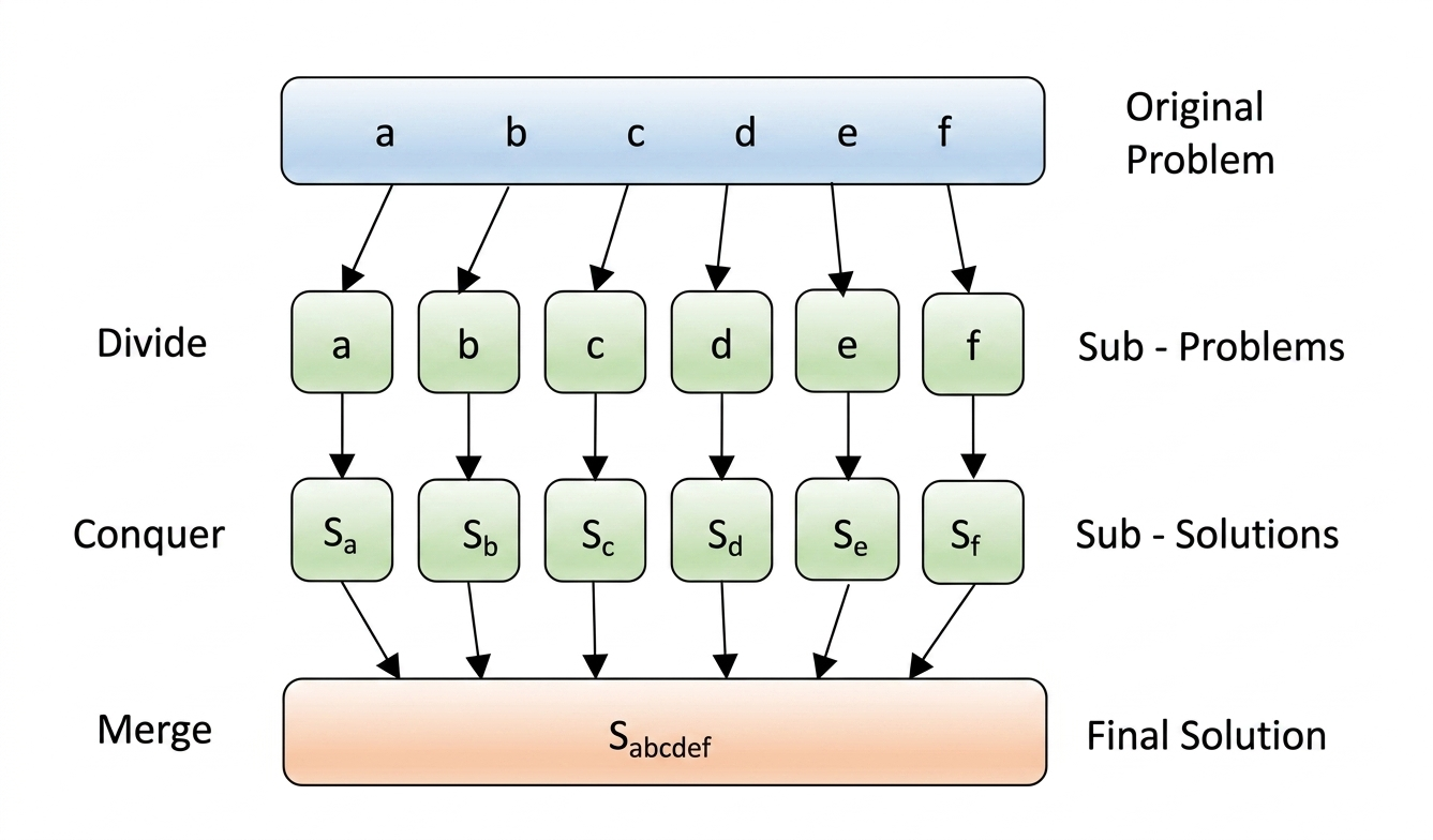
Divide and Conquer
Dynamic Programming
Greedy Algorithm
Travelling Salesman Problem (TSP):
In some versions, greedy approach selects the nearest city at each step to minimize travel cost.
Prim’s Minimum Spanning Tree:
Builds a tree by selecting the smallest edge that connects a new vertex.
Kruskal’s Minimum Spanning Tree:
Selects edges in increasing order of weight to form a minimum spanning tree.
Dijkstra’s Algorithm:
Finds the shortest path from a source vertex by always choosing the nearest unvisited vertex.
Graph Coloring:
Assigns colors to vertices such that no adjacent vertices have the same color using minimum colors.
Vertex Cover:
Selects a minimum set of vertices such that every edge is covered.
Fractional Knapsack:
Selects items based on highest value/weight ratio to maximize profit.
Job Sequencing with Deadline:
Schedules jobs to maximize profit within given deadlines.
Optimal Merge Pattern:
Combines files in such a way that total merging cost is minimized.
[urcr_restrict]
Example: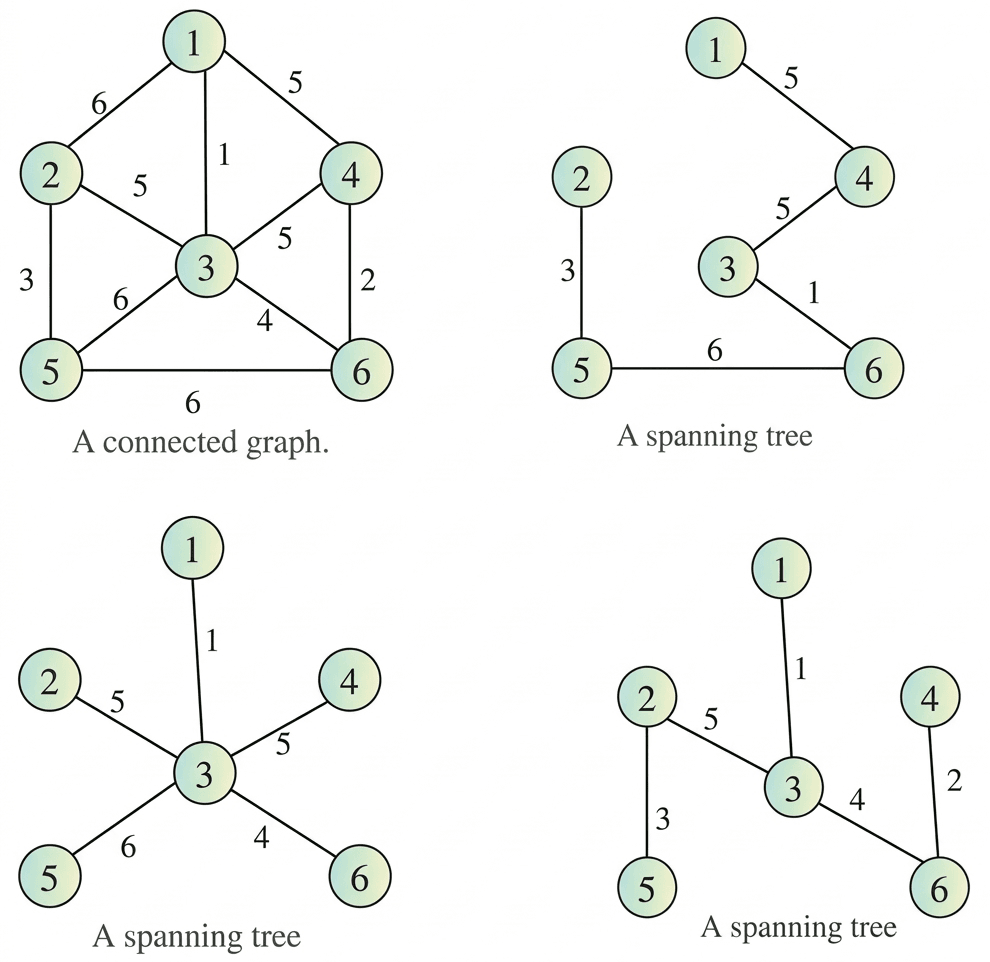
[/urcr_restrict]
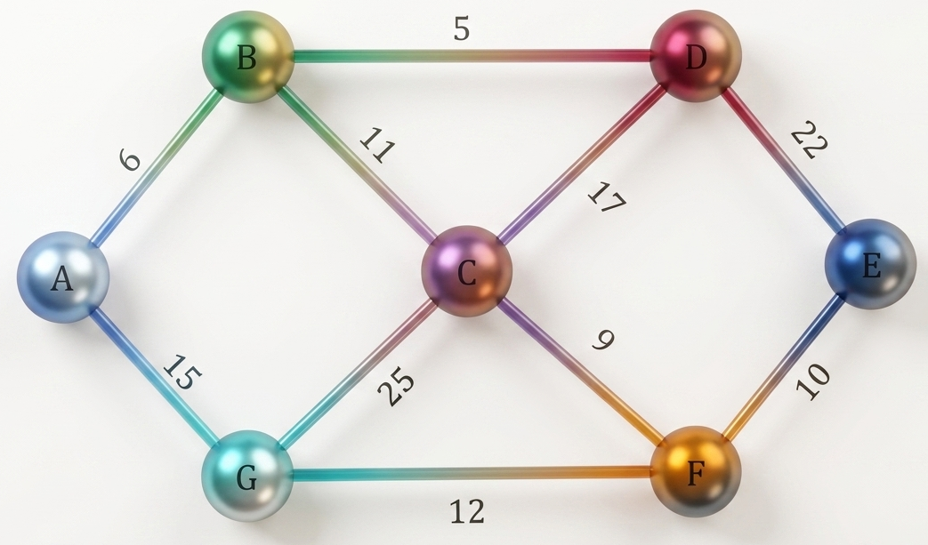
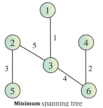
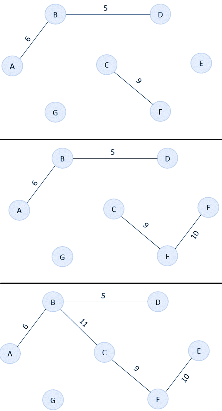
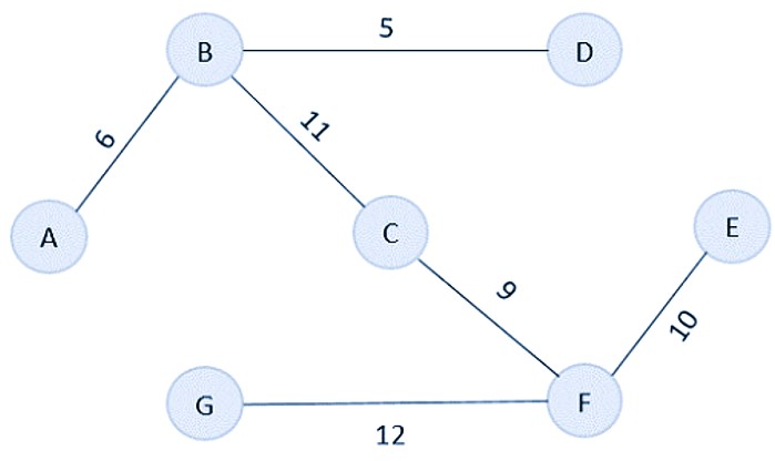
As the first step, sort all the edges in the given graph in an ascending order and store the values in an array.
Edge 	B→D 	A→B 	C→F 	F→E 	B→C 	G→F 	A→G 	C→D 	D→E 	C→G
Cost 	5 	6 	9 	10 	11 	12 	15 	17 	22 	25
Then, construct a forest of the given graph on a single plane.
From the list of sorted edge costs, select the least cost edge and add it onto the forest in output graph.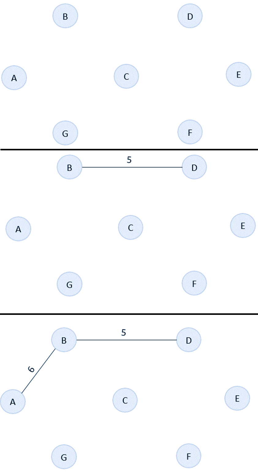
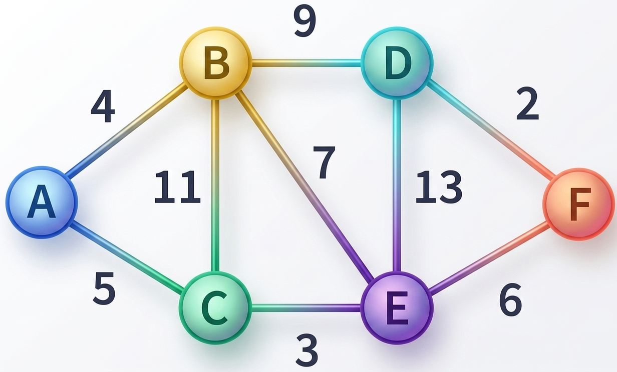
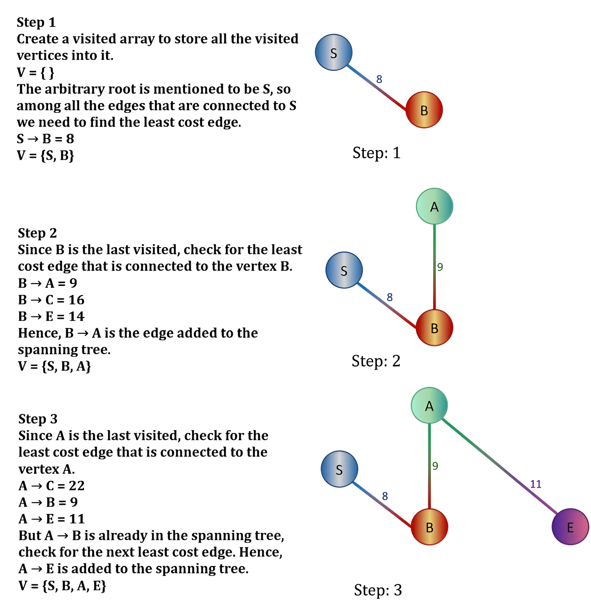
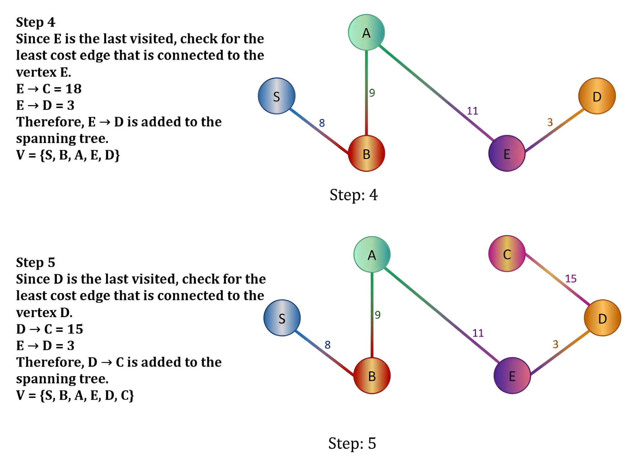
Step 1:
Visit Node A
Neighbors of A are B (weight 4) and C (weight 5).
Update B: 0+4=4
Update C: 0+5=5
Current shortest unvisited node: B (4).
Step 2:
Visit Node B
Neighbors of B are C, D, E.
Update C: min(5,4+11)=5 (No change)
Update D: 4+9=13
Update E: 4+7=11
Current shortest unvisited node: C (5).
Step 3:
Visit Node C
Neighbor of C is E.
Update E: min(11,5+3)=8
Current shortest unvisited node: E (8).
Step 4:
Visit Node E
Neighbors of E are D and F.
Update D: min(13,8+13)=13 (No change)
Update F: 8+6=14
Current shortest unvisited node: D (13).
Step 5:
Visit Node D
Neighbor of D is F.
Update F: min(14,13+2)=14 (No change)
Current shortest unvisited node: F (14).
Step 6:
Visit Node F
All nodes visited.
Reason:
- Dijkstra’s Algorithm follows a greedy approach.
- Once a vertex is marked as visited, its shortest distance is considered final.
- It does not reconsider that vertex again.
- If there is a negative weight edge, a shorter path may appear later.
- But Dijkstra cannot update it, so it gives wrong result.
Example:
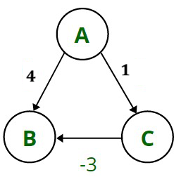
- Graph edges:
- A → B = 4
- A → C = 1
- C → B = -3
- Start from source A
- Step 1: distance(A→B) = 4, distance(A→C) = 1
- Step 2: Pick C (smallest distance = 1)
- Update B through C → distance = 1 + (-3) = -2
- But if B was already marked visited earlier, Dijkstra would keep distance = 4
- So the correct shortest path is -2, but Dijkstra may give 4 ❌
- Dijkstra fails when graph has negative weight edges.
- Bellman-Ford Algorithm is used instead in such cases.
Dijkstra’s Algorithm negative weight-এ কেন fail করে
কারণ:
- Dijkstra একটি greedy algorithm।
- একবার কোনো vertex visited হলে সেটির distance final ধরা হয়।
- পরে আর সেই vertex update করা হয় না।
- কিন্তু যদি negative weight edge থাকে, পরে আরও ছোট path পাওয়া যেতে পারে।
- Dijkstra সেটা update করতে পারে না, তাই ভুল result দেয়।
উদাহরণ:
- Graph edges:
- A → B = 4
- A → C = 1
- C → B = -3
- Source = A
- Step 1: A→B = 4, A→C = 1
- Step 2: C নির্বাচন করা হয় (distance কম = 1)
- C → B দিয়ে নতুন distance = 1 + (-3) = -2
- কিন্তু যদি B আগে visited হয়ে যায়, তাহলে Dijkstra 4-ই রেখে দেয়
- সঠিক shortest path = -2, কিন্তু Dijkstra দেয় 4 ❌
উপসংহার:
- Negative weight থাকলে Dijkstra কাজ করে না।
- এই ক্ষেত্রে Bellman-Ford Algorithm ব্যবহার করা হয়।
Previous Question with ANSWER on Design & Analysis of Algorithm(old)
Merge Sort Algorithm
Merge Sort is a divide and conquer algorithm. It recursively splits an array into two halves, sorts each half, and then merges the sorted halves back together.
Merge Sort Function
void MergeSort(int A[], int p, int r) {
    if (p < r) {
        int q = (p + r) / 2;  // Find the middle index
        MergeSort(A, p, q);    // Recursively sort the left half
        MergeSort(A, q + 1, r); // Recursively sort the right half
        merge(A, p, q, r);      // Merge the sorted halves
    }
}
Merge Function
void merge(int A[], int p, int q, int r) {
    int n1 = q - p + 1;
    int n2 = r - q;
    int L[n1], R[n2];

    // Copy data into temporary arrays
    for (int i = 0; i < n1; i++) L[i] = A[p + i];
    for (int j = 0; j < n2; j++) R[j] = A[q + 1 + j];

    int i = 0, j = 0, k = p;
    // Merge the two subarrays
    while (i < n1 && j < n2) {
        if (L[i] <= R[j]) A[k++] = L[i++];
        else A[k++] = R[j++];
    }

    // Copy remaining elements of L[]
    while (i < n1) A[k++] = L[i++];
    // Copy remaining elements of R[]
    while (j < n2) A[k++] = R[j++];
}
Dijkstra(G, s)
for each vertex v in G
    dist[v] = infinity
    visited[v] = false

dist[s] = 0

for i = 1 to number of vertices
    u = vertex with minimum dist[u] among unvisited vertices
    visited[u] = true

    for each neighbor v of u
        if visited[v] == false and dist[u] + w(u,v) < dist[v]
            dist[v] = dist[u] + w(u,v)

return dist
 Sonali Bank, O(it), 21