Basic Introduction to Database, DBMS, Types of DBMS
1. Hierarchical DBMS
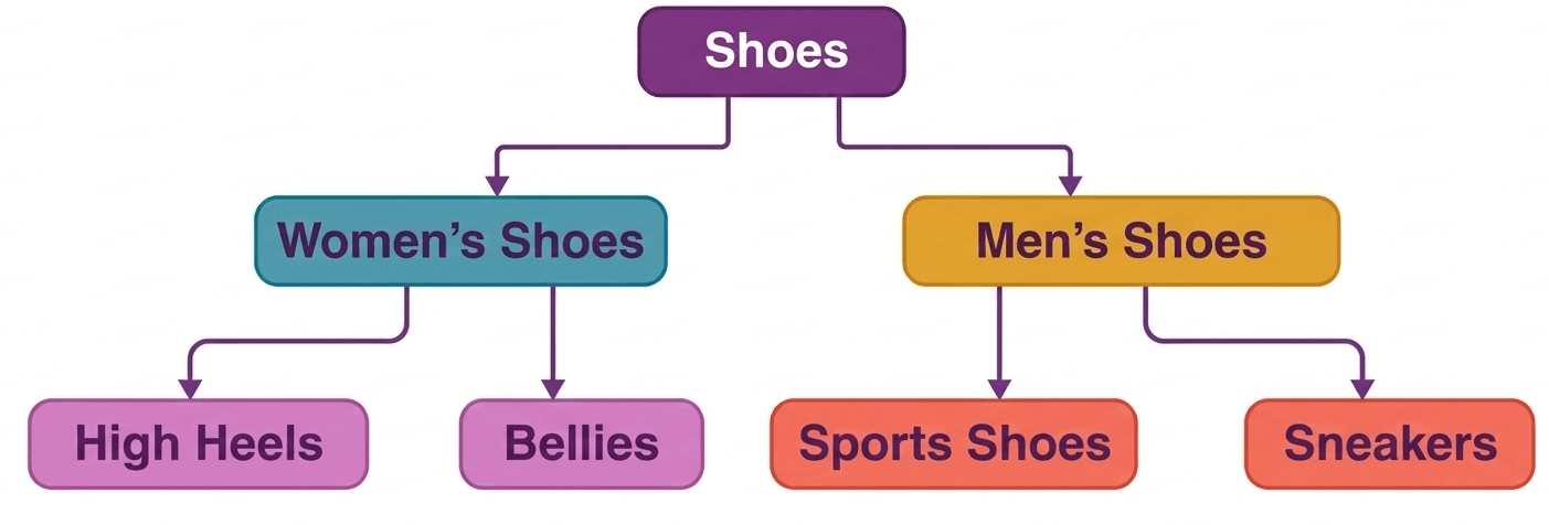
A hierarchical database management system stores data in a tree-like structure where data is organized in a parent–child relationship. Each node represents a specific entity. In this model, a parent node can have one or more child nodes, but a child node can have only one parent node. This structure supports one-to-one and one-to-many relationships. It is simple to understand but less flexible when complex relationships are needed.
2. Network DBMS
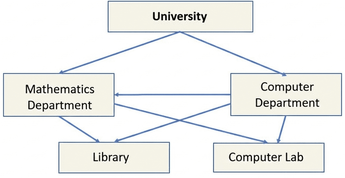
A network DBMS is an extension of the hierarchical model. It allows many-to-many relationships between entities, which makes it more flexible for representing real-life relationships. In this model, records are connected using links or pointers and the relationships between nodes are represented by arrows. This structure allows a child node to have multiple parent nodes, improving data accessibility and flexibility.
3. Relational DBMS (RDBMS)
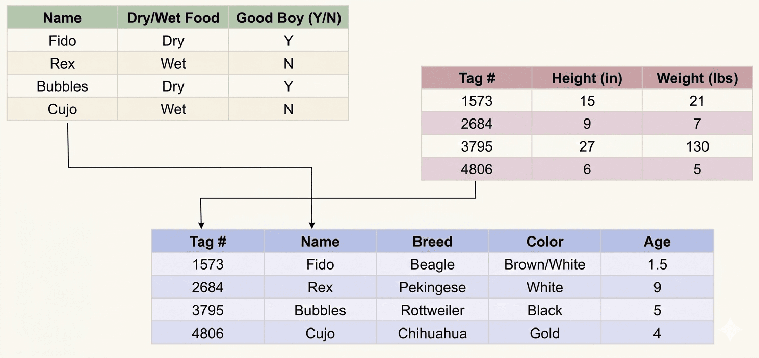
A relational database management system stores data in the form of tables, also known as relations. Each table consists of rows and columns where rows represent records and columns represent attributes. Relationships between tables are established using keys such as primary key and foreign key. This model is widely used because it is simple, flexible, and allows efficient data management using SQL.
4. Object-Oriented DBMS (OODBMS)
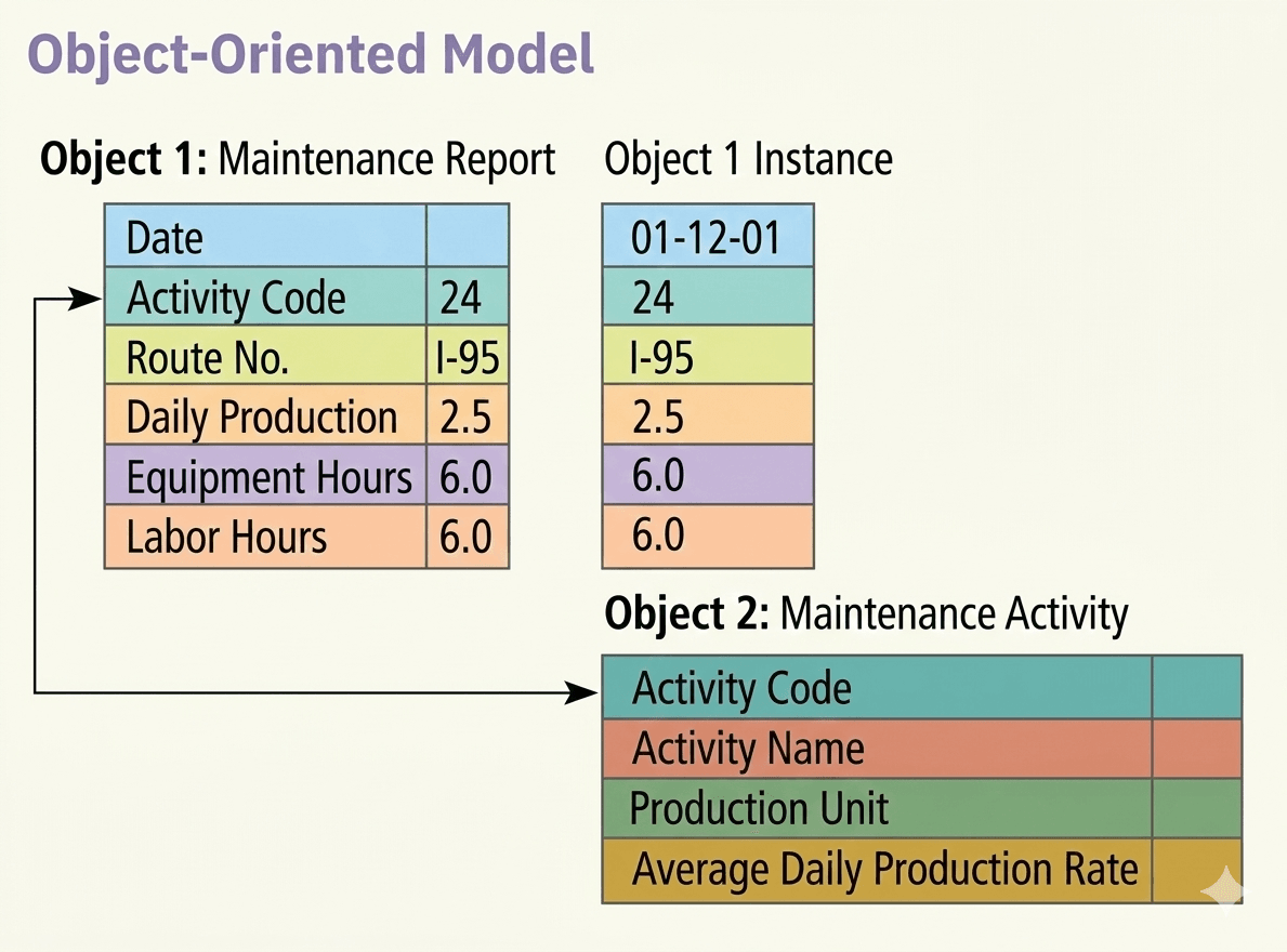
An object-oriented database management system is based on the concepts of object-oriented programming (OOP). In this model, data is stored in the form of objects instead of tables. Objects contain both data and methods that operate on the data. This system supports programming languages such as Java, C++, .NET, and Visual Basic and provides a unified environment for storing and managing complex data.
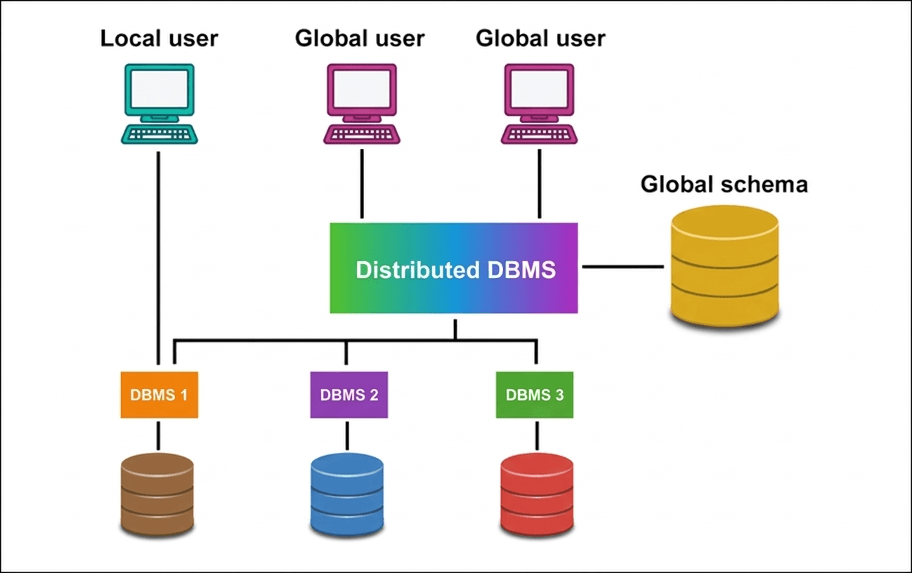
5. Distributed DBMS (DDBMS)
A distributed database management system stores data across multiple computers or nodes connected through a network. Instead of storing all data in a single location, the data is divided and distributed across different physical or logical locations. The management of the database is decentralized, which improves data availability, reliability, and performance in large-scale systems.
1. Hierarchical DBMS
Hierarchical DBMS-এ data একটি tree structure-এর মতো parent–child relationship আকারে সংরক্ষিত হয়। এখানে প্রতিটি node একটি নির্দিষ্ট entity নির্দেশ করে। একটি parent node-এর এক বা একাধিক child node থাকতে পারে, কিন্তু একটি child node-এর শুধুমাত্র একটি parent node থাকে। এই model one-to-one এবং one-to-many relationship সমর্থন করে। এটি বুঝতে সহজ হলেও complex relationship পরিচালনায় সীমাবদ্ধতা রয়েছে।
2. Network DBMS
Network DBMS hierarchical model-এর একটি উন্নত রূপ। এটি many-to-many relationship সমর্থন করে, যা বাস্তব জীবনের বিভিন্ন entity-এর মধ্যে সম্পর্ক সংরক্ষণে সাহায্য করে। এই model-এ record-গুলোর মধ্যে link বা pointer ব্যবহার করে সংযোগ তৈরি করা হয় এবং node-গুলোর সম্পর্ক arrow দ্বারা দেখানো হয়। এখানে একটি child node একাধিক parent node-এর সাথে সম্পর্কিত হতে পারে, যা database design-কে আরও flexible করে।
3. Relational DBMS (RDBMS)
Relational DBMS-এ data table আকারে সংরক্ষিত হয়, যাকে relation বলা হয়। প্রতিটি table-এ row এবং column থাকে যেখানে row একটি record এবং column একটি attribute নির্দেশ করে। বিভিন্ন table-এর মধ্যে relationship primary key এবং foreign key ব্যবহার করে তৈরি করা হয়। এই model খুব জনপ্রিয় কারণ এটি সহজ, flexible এবং SQL ব্যবহার করে data সহজে পরিচালনা করা যায়।
4. Object-Oriented DBMS (OODBMS)
Object-Oriented DBMS object-oriented programming (OOP)-এর ধারণার উপর ভিত্তি করে তৈরি। এখানে data table-এর পরিবর্তে object আকারে সংরক্ষিত হয়। একটি object-এর মধ্যে data এবং সেই data পরিচালনার method উভয়ই থাকে। এই system Java, C++, .NET এবং Visual Basic-এর মতো programming language-এর সাথে সহজে কাজ করতে পারে এবং complex data পরিচালনার জন্য উপযোগী।
5. Distributed DBMS (DDBMS)
Distributed DBMS-এ data একাধিক computer বা node-এ network-এর মাধ্যমে সংরক্ষিত থাকে। সব data একটি স্থানে না রেখে বিভিন্ন physical বা logical location-এ ভাগ করে রাখা হয়। এই system-এ database management decentralized থাকে, যার ফলে data availability, reliability এবং performance বৃদ্ধি পায়।
Data Abstraction, Data Model: (ER Model, Relational Model, Object Oriented Model) & Database Architecture
As the name suggests, the object-oriented data model combines the principles of object-oriented programming with database concepts. In this model, both data and their relationships are grouped together into a single structure called an object.
Because data is stored as objects, it becomes easier to store complex data types such as audio, video, images, and multimedia files, which was challenging to handle in the traditional relational model.
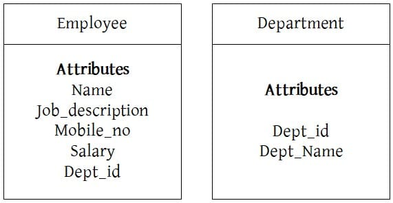
For example, consider two objects — Employee and Department. Each object contains all relevant data in a single unit, and they are connected through a link based on a shared attribute, such as Department_ID.
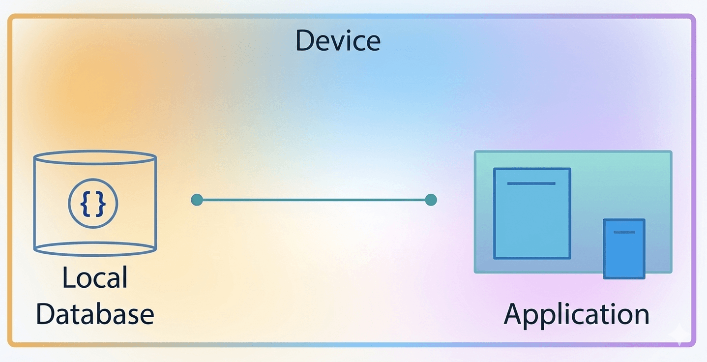
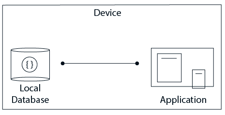
One-Tier (Single-Tier) Architecture
In this architecture, the database is directly accessible to the user. The user works directly on the DBMS, and any changes made are immediately applied to the database.
However, this architecture does not provide a user-friendly interface for end-users. It is mainly used during application development, where programmers require quick and direct access to the database for testing and development.
Single-Tier Architecture is suitable when:
- The data does not change frequently.
- There is no need for multiple users to access the database at the same time.
- A simple and direct way to access or modify the database is required (e.g., during development).
Example: When learning SQL, we often install a database server (such as SQL Server, MySQL, or Oracle) on our local system. We can directly interact with the database and run queries without a network connection. This is a practical example of Single-Tier Architecture.
In conclusion, One-Tier Architecture is simple and suitable for development and local use but not ideal for large multi-user systems.
One-Tier (Single-Tier) Architecture
এই Architecture-এ Database সরাসরি User দ্বারা Access করা যায়। User সরাসরি DBMS-এ কাজ করে এবং যেকোনো পরিবর্তন সাথে সাথে Database-এ প্রয়োগ হয়।
তবে এই Architecture End-User-এর জন্য খুব User-friendly Interface প্রদান করে না। এটি মূলত Application Development-এর সময় ব্যবহৃত হয়, যেখানে Programmer দ্রুত ও সরাসরি Database Access করে Testing ও Development করতে চায়।
Single-Tier Architecture উপযুক্ত যখন:
- Data ঘন ঘন পরিবর্তন হয় না।
- একাধিক User একসাথে Database ব্যবহার করার প্রয়োজন নেই।
- Development-এর সময় সরাসরি ও সহজভাবে Database Access বা Modify করার প্রয়োজন হয়।
উদাহরণ: SQL শেখার সময় আমরা অনেক সময় Local System-এ Database Server (যেমন SQL Server, MySQL, Oracle) Install করি। এতে Network ছাড়াই সরাসরি Database-এর সাথে Interaction করে Query চালানো যায়। এটি Single-Tier Architecture-এর একটি বাস্তব উদাহরণ।
সারসংক্ষেপে, One-Tier Architecture সহজ ও Development-এর জন্য উপযোগী, তবে বড় Multi-user System-এর জন্য উপযুক্ত নয়।
[/urcr_restrict]
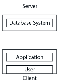
Two-Tier Architecture
The Two-Tier Architecture follows the Client–Server Model. In this architecture, the application running on the client side directly communicates with the database server.
Technologies such as ODBC (Open Database Connectivity) and JDBC (Java Database Connectivity) are commonly used to establish this connection.
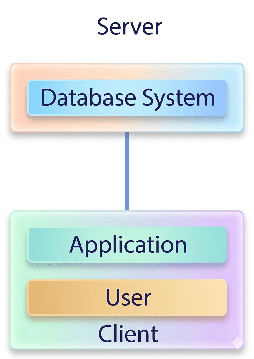
In this architecture:
- The client side handles the User Interface and Application Logic.
- The server side manages Query Processing, Transaction Management, and database operations.
- The client establishes a direct connection with the server to perform operations such as Retrieve, Insert, Update, and Delete.
Advantages of Two-Tier Architecture:
- Supports multiple users simultaneously.
- Offers better performance as the server independently processes database operations.
- Provides faster access due to direct client-server communication.
- Easier maintenance because the system is divided into two layers.
Example: When visiting a bank to withdraw money, the banker uses a computer (client) to send a request to the bank’s database server. The server checks your balance and sends the response back. This is a real-life example of Two-Tier Architecture.
In conclusion, Two-Tier Architecture improves performance and supports multiple users but depends on direct client-server communication.
Two-Tier Architecture
Two-Tier Architecture হলো Client–Server Model ভিত্তিক একটি Architecture। এখানে Client Side-এর Application সরাসরি Database Server-এর সাথে যোগাযোগ করে।
ODBC (Open Database Connectivity) এবং JDBC (Java Database Connectivity) প্রযুক্তি ব্যবহার করে এই সংযোগ স্থাপন করা হয়।
এই Architecture-এ:
- Client Side User Interface ও Application Logic পরিচালনা করে।
- Server Side Query Processing, Transaction Management এবং Database Operation পরিচালনা করে।
- Client সরাসরি Server-এর সাথে Connection স্থাপন করে Retrieve, Insert, Update ও Delete Operation সম্পাদন করে।
Two-Tier Architecture-এর সুবিধাসমূহ:
- একাধিক User একই সময়ে System ব্যবহার করতে পারে।
- Server আলাদাভাবে Database Process করায় Performance ভালো হয়।
- Direct Client-Server Communication হওয়ায় দ্রুত Data Access পাওয়া যায়।
- দুইটি Layer থাকায় Maintenance তুলনামূলক সহজ।
উদাহরণ: ব্যাংকে টাকা তুলতে গেলে Banker Computer (Client) ব্যবহার করে Database Server-এ Request পাঠায়। Server Balance যাচাই করে Response পাঠায়। এটি Two-Tier Architecture-এর একটি বাস্তব উদাহরণ।
সারসংক্ষেপে, Two-Tier Architecture Performance উন্নত করে এবং একাধিক User সমর্থন করে, তবে এটি সরাসরি Client-Server Connection-এর উপর নির্ভরশীল।
[/urcr_restrict]
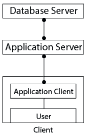
Three-Tier Architecture
The Three-Tier Architecture introduces an additional layer between the client and the database server. In this setup, the client does not directly communicate with the database.
Instead, the client interacts with an Application Server (Middleware), which processes the request and communicates with the database server.
In this architecture:
- Client Layer: Responsible for the User Interface.
- Application Layer: Contains Business Logic and handles client requests.
- Database Layer: Manages data storage, retrieval, and processing.
This architecture is widely used in large-scale web applications because it improves manageability, scalability, and security.
Advantages of Three-Tier Architecture:
1. Scalability: The application layer supports load balancing, allowing multiple clients without affecting database performance.
2. Data Integrity: The application layer validates requests before sending them to the database, reducing invalid data.
3. Security: Direct access between client and database is removed, increasing data protection.
In conclusion, Three-Tier Architecture provides better security, scalability, and control but increases system complexity.
Three-Tier Architecture
Three-Tier Architecture-এ Client ও Database Server-এর মাঝে একটি অতিরিক্ত Layer যুক্ত হয়। এখানে Client সরাসরি Database-এর সাথে যোগাযোগ করে না।
Client একটি Application Server (Middleware)-এর সাথে যোগাযোগ করে, এবং Application Server Database Server-এর সাথে যোগাযোগ করে Data আদান-প্রদান সম্পন্ন করে।
এই Architecture-এ:
- Client Layer: User Interface পরিচালনা করে।
- Application Layer: Business Logic ধারণ করে এবং Client Request Process করে।
- Database Layer: Data Storage, Retrieval ও Processing পরিচালনা করে।
বড় Web Application-এ এই Architecture বেশি ব্যবহৃত হয়, কারণ এটি Manageability, Scalability ও Security উন্নত করে।
Three-Tier Architecture-এর সুবিধাসমূহ:
১. Scalability: Application Layer Load Balancing সমর্থন করে, ফলে একাধিক Client যুক্ত হলেও Database Performance প্রভাবিত হয় না।
২. Data Integrity: Application Layer Database-এ পাঠানোর আগে Request Validate করে, ফলে Invalid Data কমে।
৩. Security: Client ও Database-এর সরাসরি সংযোগ না থাকায় Unauthorized Access কঠিন হয়।
সারসংক্ষেপে, Three-Tier Architecture উন্নত Security ও Scalability প্রদান করে, তবে System Design আরও Complex হয়।
[/urcr_restrict]
Data Abstraction in DBMS
Data Abstraction is an important concept in DBMS. It means hiding unnecessary and complex details from users and showing only the required information.
Users can access the needed data without knowing how the data is stored in the database.
- Hiding Complexity: Data abstraction hides internal database details from the user.
- Security: It protects data by hiding how and where the data is stored.
- Simplified Access: Users can easily access necessary data without understanding the database structure.
- Example: When buying clothes online, users only see color, size, and brand, but not the manufacturing details.
Levels of Data Abstraction in DBMS
There are three levels of data abstraction in DBMS:
- Physical (Internal) Level
- Logical (Conceptual) Level
- View (External) Level
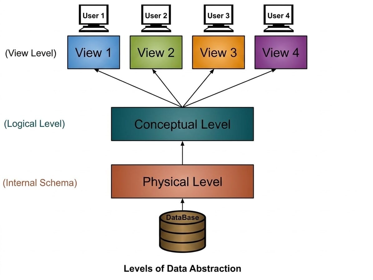
1. Physical or Internal Level
- This is the lowest level of data abstraction.
- It describes how data is actually stored in the database.
- It includes storage details such as file structure, disk space allocation, and access methods.
- This level is very complex and usually handled by the Database Administrator (DBA).
- Users cannot see this level.
2. Logical or Conceptual Level
- This is the middle level of data abstraction.
- It describes what data is stored in the database and the relationships between them.
- It defines tables, attributes, relationships, and constraints.
- Programmers and database designers usually work at this level.
3. View or External Level
- This is the highest level of data abstraction.
- It shows only a specific part of the database required by a particular user.
- Different users can have different views of the same database.
- This level is the easiest for users to understand.
DBMS-এ Data Abstraction
Data Abstraction হলো DBMS-এর একটি গুরুত্বপূর্ণ concept। এর অর্থ হলো অপ্রয়োজনীয় ও জটিল তথ্য ব্যবহারকারীর কাছ থেকে লুকিয়ে রাখা এবং শুধু প্রয়োজনীয় তথ্য দেখানো।
এর ফলে user ডেটা ব্যবহার করতে পারে কিন্তু ডেটা কীভাবে database-এ সংরক্ষিত আছে তা দেখতে পারে না।
- Hiding Complexity: Data abstraction database-এর জটিল internal detail user থেকে লুকিয়ে রাখে।
- Security: ডেটা কোথায় এবং কীভাবে সংরক্ষিত আছে তা লুকিয়ে রেখে data security নিশ্চিত করে।
- Simplified Access: User সহজে প্রয়োজনীয় data access করতে পারে।
- উদাহরণ: Online-এ কাপড় কিনতে গেলে user শুধু color, size এবং brand দেখে, কিন্তু production detail দেখে না।
DBMS-এ Data Abstraction-এর Levels
DBMS-এ তিনটি level রয়েছে:
- Physical (Internal) Level
- Logical (Conceptual) Level
- View (External) Level
1. Physical বা Internal Level
- এটি data abstraction-এর সবচেয়ে নিচের level।
- এখানে database-এ data কীভাবে store করা হয় তা নির্ধারণ করা হয়।
- এতে file structure, disk space allocation এবং data access method অন্তর্ভুক্ত থাকে।
- এই level খুব complex এবং সাধারণত Database Administrator (DBA) এটি পরিচালনা করে।
- User এই level দেখতে পারে না।
2. Logical বা Conceptual Level
- এটি data abstraction-এর মাঝামাঝি level।
- এখানে database-এ কোন data থাকবে এবং তাদের relationship কী হবে তা নির্ধারণ করা হয়।
- এতে table structure, attribute, relationship এবং constraint নির্ধারণ করা হয়।
- Programmer এবং database designer সাধারণত এই level-এ কাজ করে।
3. View বা External Level
- এটি data abstraction-এর সর্বোচ্চ level।
- এখানে user-এর জন্য database-এর একটি নির্দিষ্ট অংশ দেখানো হয়।
- একই database-এর বিভিন্ন user-এর জন্য বিভিন্ন view থাকতে পারে।
- এটি user-এর জন্য সবচেয়ে সহজ level।
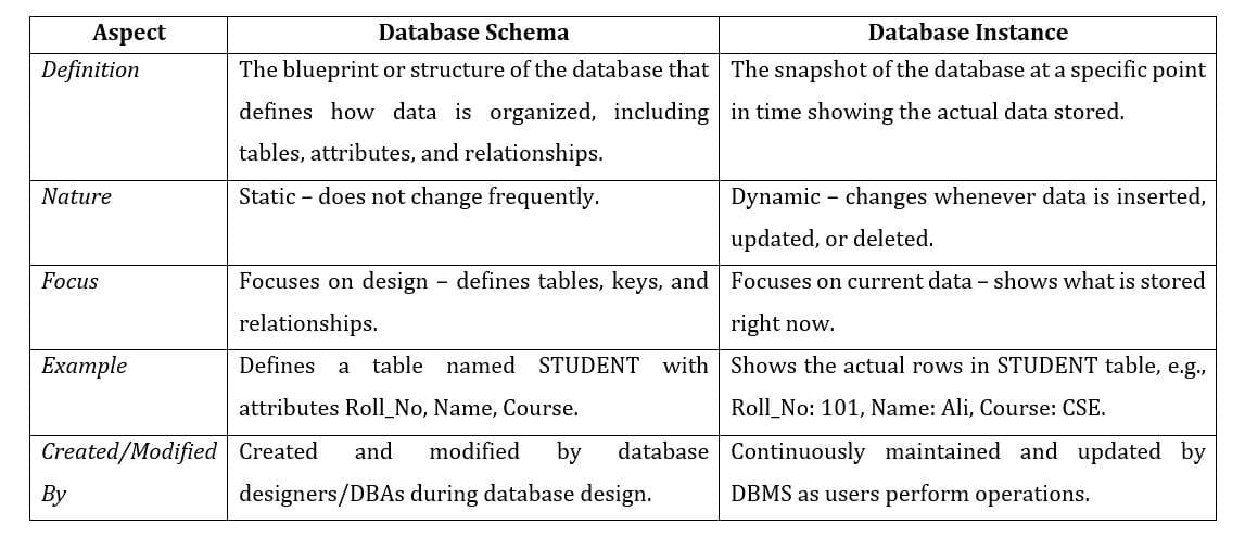
Database Schema & Database Instance
A Database Schema is the blueprint or skeleton structure of a database that represents its logical view. It defines how data is organized, how entities are related, and what constraints are applied to the data.
A schema describes the Entities, their Attributes, and the Relationships among them. This structure is often shown using a Schema Diagram.
Database designers create the schema so that developers and programmers can clearly understand the database structure.
In an RDBMS (Relational Database Management System), data is logically represented in the form of tables (relations).
In an E-R Model, data is represented using entities and relationships.
Example: To store student details, a STUDENT table can be created with attributes such as Roll Number, Name, Course, etc.
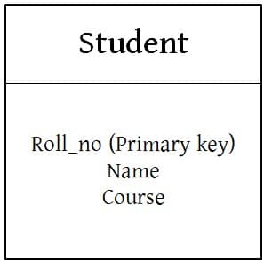
A schema does not include low-level details like data types. Instead, it focuses on logical constraints such as tables, Primary Keys, and relationships among tables.
In conclusion, Database Schema provides the logical structure of a database and guides its proper design and implementation.
Database Schema হলো একটি Database-এর Blueprint বা Skeleton Structure, যা এর Logical View উপস্থাপন করে। এটি নির্ধারণ করে Data কীভাবে সংগঠিত হবে, Entity গুলোর মধ্যে কী সম্পর্ক থাকবে এবং কী ধরনের Constraint প্রয়োগ হবে।
Schema-তে Entity, তাদের Attribute এবং Relationship বিস্তারিতভাবে বর্ণনা করা হয়। এটি সাধারণত Schema Diagram আকারে উপস্থাপন করা হয়।
Database Designer Schema তৈরি করেন যাতে Developer ও Programmer সহজে Database Structure বুঝতে পারে।
RDBMS (Relational Database Management System)-এ Data Table (Relation) আকারে Logicalভাবে উপস্থাপিত হয়।
E-R Model-এ Data Entity ও Relationship ব্যবহার করে উপস্থাপন করা হয়।
উদাহরণ: Student-এর তথ্য সংরক্ষণের জন্য STUDENT নামে একটি Table তৈরি করা যায়, যেখানে Roll Number, Name, Course ইত্যাদি Attribute থাকবে।
Schema-তে Attribute-এর Data Type-এর মতো Low-level Detail দেখানো হয় না। বরং এটি Logical Constraint যেমন Table, Primary Key এবং Relationship-এর উপর গুরুত্ব দেয়।
সারসংক্ষেপে, Database Schema Database-এর Logical Structure নির্ধারণ করে এবং সঠিকভাবে Design ও Implementation করতে সহায়তা করে।
[urcr_restrict]
[/urcr_restrict]
Relational Model & Contsraints in Relational Model
Keys in Database
In a Relational Database Management System (RDBMS), keys are very important because they help uniquely identify records and establish relationships between tables. Keys also prevent duplicate data and maintain data integrity. The following are the major types of keys used in RDBMS.
1. Super Key
A Super Key is any set of one or more attributes that can uniquely identify a record in a table. A super key may include additional attributes that are not necessary for identification.
Example Table: Student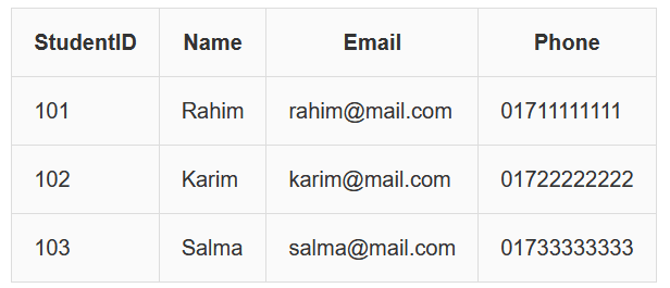
Possible Super Keys:
{StudentID}
{StudentID, Name}
{StudentID, Email}
{StudentID, Name, Phone}
Explanation: StudentID alone uniquely identifies a student. Adding extra attributes like Name or Phone still keeps the record unique, so those combinations are also super keys.
2. Candidate Key
A Candidate Key is a minimal Super Key. It means the key contains only the necessary attributes required to uniquely identify a record. Removing any attribute will break the uniqueness.
Example Table: Student
| StudentID | Name | |
|---|---|---|
| 101 | Rahim | rahim@mail.com |
| 102 | Karim | karim@mail.com |
| 103 | Salma | salma@mail.com |
Possible Candidate Keys:
{StudentID}
{Email}
Explanation: Both StudentID and Email uniquely identify each student. Since neither needs extra attributes, they are minimal super keys and therefore candidate keys.
3. Primary Key
A Primary Key is the candidate key selected by the database designer to uniquely identify each record in the table. A primary key must always be unique and cannot contain NULL values.
Example Table: Student
| StudentID (Primary Key) | Name | |
|---|---|---|
| 101 | Rahim | rahim@mail.com |
| 102 | Karim | karim@mail.com |
| 103 | Salma | salma@mail.com |
Explanation: In this table, StudentID is chosen as the primary key because it uniquely identifies each student and does not contain duplicate or NULL values.
4. Alternate Key
An Alternate Key is a candidate key that was not selected as the primary key. It can still uniquely identify records but is not used as the main identifier.
Example Table: Student
| StudentID (PK) | Name | Email (Alternate Key) |
|---|---|---|
| 101 | Rahim | rahim@mail.com |
| 102 | Karim | karim@mail.com |
| 103 | Salma | salma@mail.com |
Explanation: Email is unique for every student but since StudentID is selected as the primary key, Email becomes the alternate key.
5. Unique Key
A Unique Key ensures that all values in a column are unique across the table. Some DBMS allow NULL values in unique keys, but duplicate values are not allowed.
Example Table: Student
| StudentID | Name | Email (Unique) |
|---|---|---|
| 101 | Rahim | rahim@mail.com |
| 102 | Karim | karim@mail.com |
| 103 | Salma | salma@mail.com |
Explanation: The Email column is marked as UNIQUE. Therefore, no two students can have the same email address.
6. Composite Key
A Composite Key is a key formed by combining two or more attributes to uniquely identify a record. It is used when a single column cannot uniquely identify a record.
Example Table: Enrollment
| StudentID | CourseID | Semester |
|---|---|---|
| 101 | CSE101 | Spring |
| 101 | CSE102 | Spring |
| 102 | CSE101 | Fall |
Composite Key:
{StudentID, CourseID}
Explanation: A student can take multiple courses and a course can have multiple students. So neither StudentID nor CourseID alone is unique. But together they uniquely identify each enrollment record.
7. Foreign Key
A Foreign Key is a column in one table that refers to the Primary Key of another table. It creates a relationship between the tables and ensures referential integrity.
Student Table
| StudentID (PK) | Name |
|---|---|
| 101 | Rahim |
| 102 | Karim |
Enrollment Table
| EnrollmentID | StudentID (Foreign Key) | CourseID |
|---|---|---|
| 1 | 101 | CSE101 |
| 2 | 102 | CSE102 |
Explanation: StudentID in the Enrollment table references StudentID in the Student table. This ensures that enrollment records cannot exist for students who are not in the Student table.
Relational Database Management System (RDBMS)-এ Key ব্যবহার করা হয় একটি table-এর record uniquely identify করার জন্য এবং বিভিন্ন table-এর মধ্যে relationship তৈরি করার জন্য। Keys database-এ data duplication কমায় এবং data integrity বজায় রাখে।
১. Super Key
Super Key হলো এক বা একাধিক attribute-এর সমষ্টি যা একটি table-এর প্রতিটি record uniquely identify করতে পারে। এতে প্রয়োজনের চেয়ে বেশি attribute থাকতে পারে।
Example Table: Student
Possible Super Keys:
{StudentID}, {StudentID, Name}, {StudentID, Email}
Explanation: StudentID একাই একজন student-কে uniquely identify করে। Name বা Email যোগ করলেও record unique থাকে।
২. Candidate Key
Candidate Key হলো minimal Super Key। অর্থাৎ কোনো attribute বাদ দিলে uniqueness নষ্ট হয়ে যাবে।
Example Table: Student
| StudentID | Name | |
|---|---|---|
| 101 | Rahim | rahim@mail.com |
| 102 | Karim | karim@mail.com |
| 103 | Salma | salma@mail.com |
Candidate Keys:
{StudentID}, {Email}
Explanation: StudentID এবং Email দুটোই unique হওয়ায় এগুলো Candidate Key।
৩. Primary Key
Primary Key হলো Candidate Key-এর মধ্য থেকে নির্বাচিত key যা record uniquely identify করে এবং NULL হতে পারে না।
Example Table
| StudentID (Primary Key) | Name | |
|---|---|---|
| 101 | Rahim | rahim@mail.com |
| 102 | Karim | karim@mail.com |
| 103 | Salma | salma@mail.com |
Explanation: StudentID প্রতিটি record uniquely identify করে।
৪. Alternate Key
Alternate Key হলো সেই Candidate Key যা Primary Key হিসেবে নির্বাচিত হয়নি।
Example
| StudentID (PK) | Name | Email (Alternate Key) |
|---|---|---|
| 101 | Rahim | rahim@mail.com |
| 102 | Karim | karim@mail.com |
| 103 | Salma | salma@mail.com |
Explanation: StudentID Primary Key হলে Email Alternate Key হয়।
৫. Unique Key
Unique Key নিশ্চিত করে যে column-এর সব value unique থাকবে।
Example
| StudentID | Name | Email (Unique) |
|---|---|---|
| 101 | Rahim | rahim@mail.com |
| 102 | Karim | karim@mail.com |
| 103 | Salma | salma@mail.com |
Explanation: Email column-এ duplicate value থাকতে পারবে না।
৬. Composite Key
Composite Key একাধিক attribute নিয়ে গঠিত যা একসাথে record uniquely identify করে।
Example Table: Enrollment
| StudentID | CourseID | Semester |
|---|---|---|
| 101 | CSE101 | Spring |
| 101 | CSE102 | Spring |
| 102 | CSE101 | Fall |
Composite Key = {StudentID, CourseID}
Explanation: StudentID বা CourseID একাই unique নয়, কিন্তু দুটো একসাথে unique।
৭. Foreign Key
Foreign Key হলো একটি table-এর attribute যা অন্য table-এর Primary Key-এর সাথে সম্পর্ক তৈরি করে।
Student Table
| StudentID (PK) | Name |
|---|---|
| 101 | Rahim |
| 102 | Karim |
Enrollment Table
| EnrollmentID | StudentID (Foreign Key) | CourseID |
|---|---|---|
| 1 | 101 | CSE101 |
| 2 | 102 | CSE102 |
Explanation: Enrollment table-এর StudentID → Student table-এর StudentID কে reference করে।
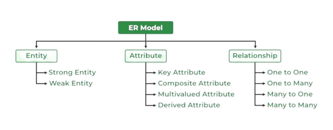
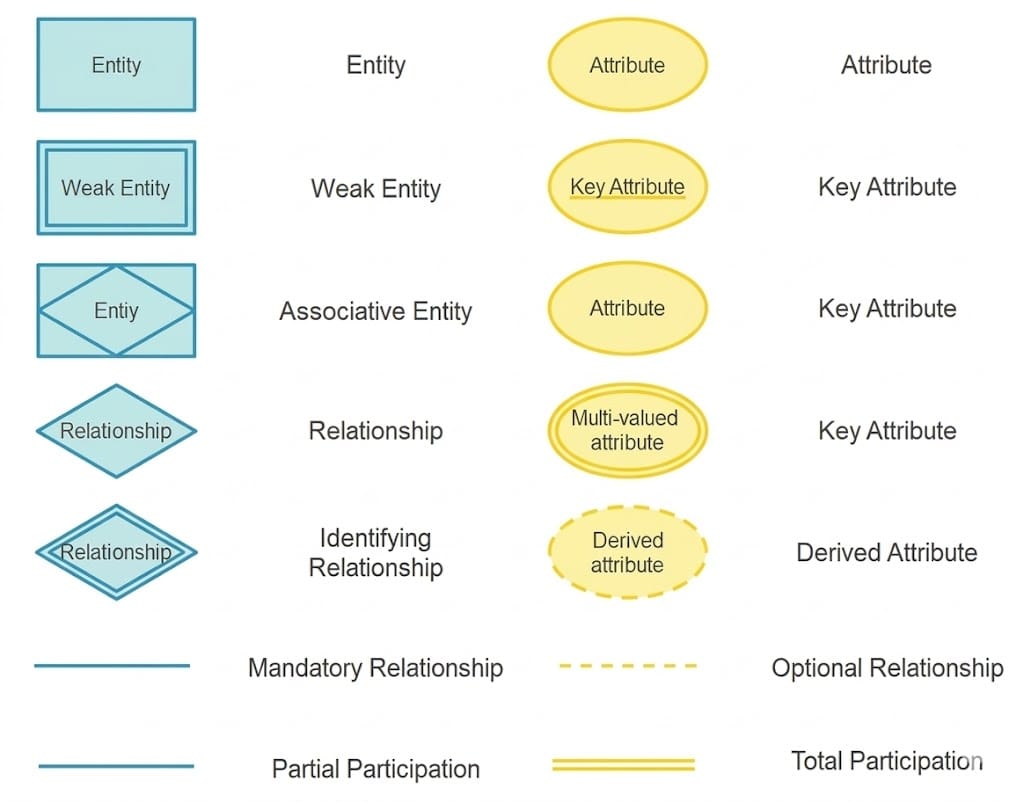
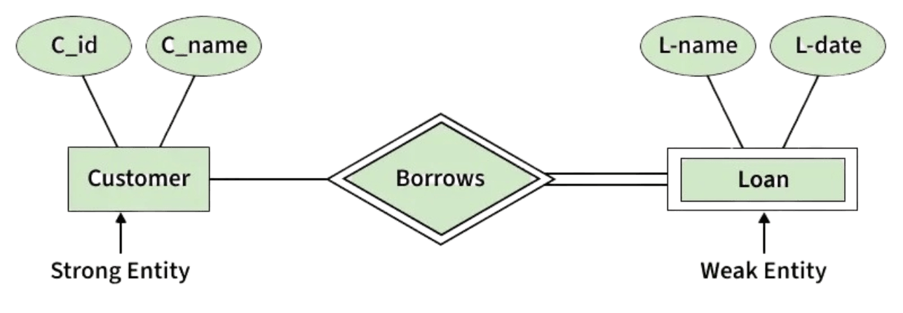
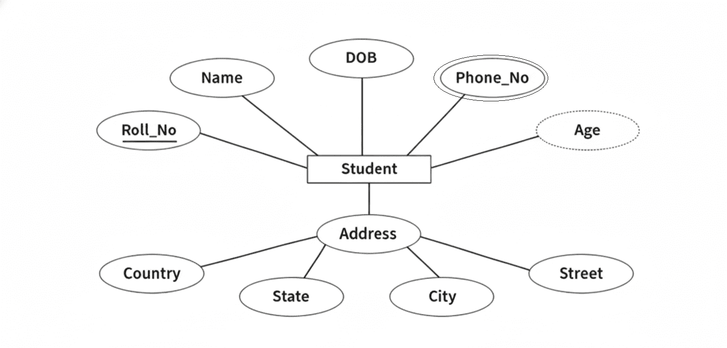
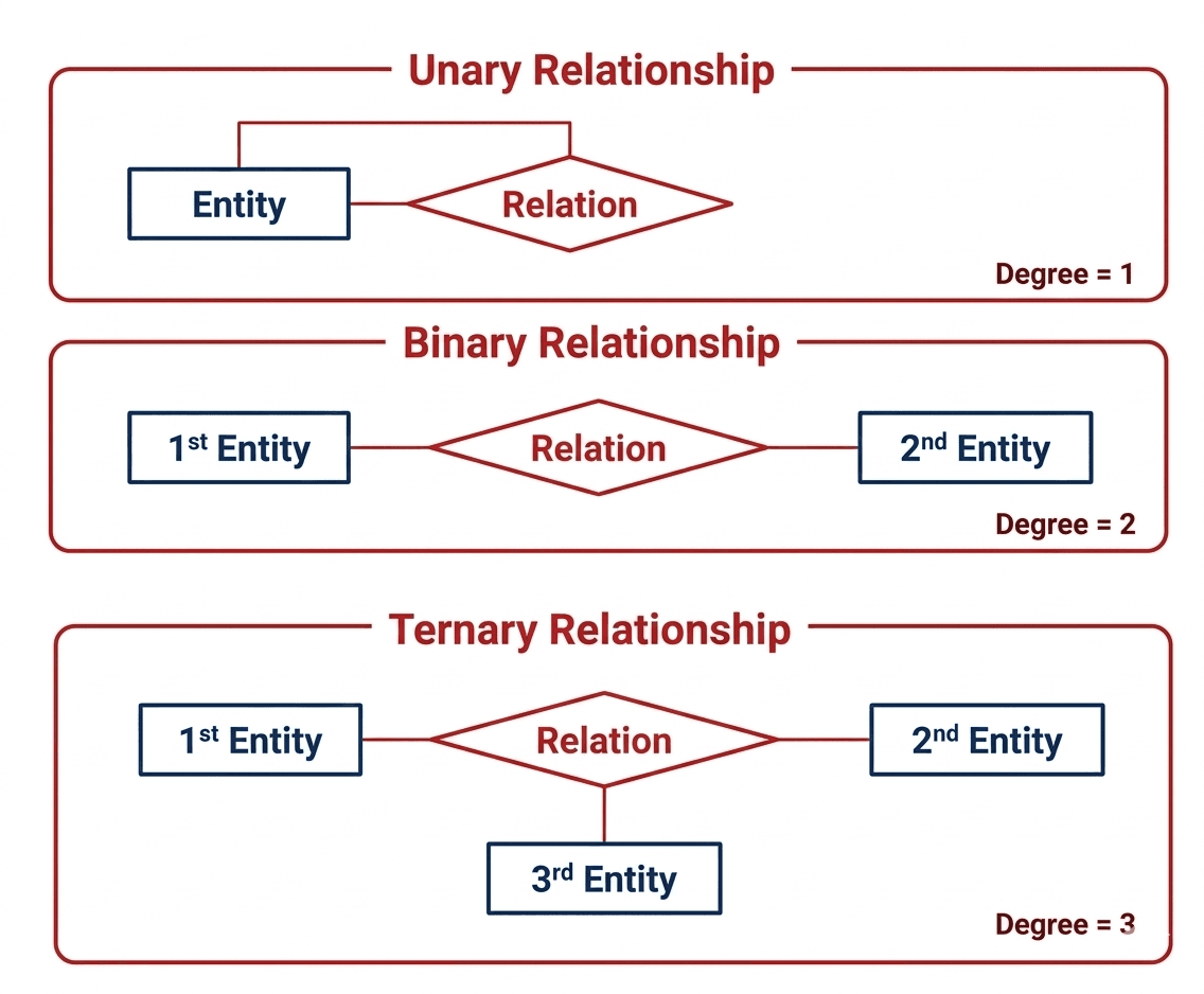
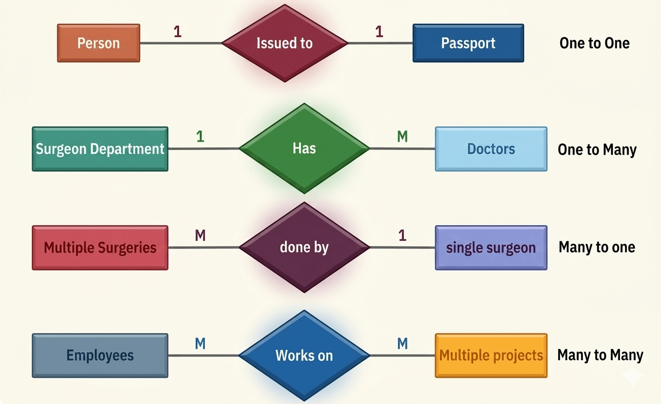
ER Model, ER Diagram, Relationship
Database Normalization
Functional Dependency in DBMS
In a Relational Database Management System (RDBMS), data is stored in the form of tables.
Each table consists of rows and columns. Columns represent the attributes (characteristics of data), while each row represents a record.
Every row in a table has the same structure and a row is also called a tuple in DBMS.
Example: Employee Table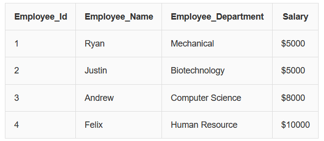
From this table we can observe that Employee_Id uniquely identifies each employee.
If we know the Employee_Id, we can determine the employee’s name, department and salary.
Definition of Functional Dependency
A Functional Dependency (FD) describes the relationship between attributes in a table.
It means that the value of one attribute determines the value of another attribute.
Functional dependency is written using the arrow symbol:
X → Y
This means attribute X determines attribute Y.
Example:
Employee_Id → Employee_Name, Employee_Department, Salary
This means if we know the Employee_Id, we can determine the employee’s name, department and salary.
Example Relation
Suppose we have a relation:
R(A, B, C, D)
Possible Functional Dependencies:
A → BCD
B → CD
Explanation:
• In A → BCD, attribute A determines attributes B, C and D.
• In B → CD, attribute B determines attributes C and D.
In Functional Dependency:
• The left side is called the Determinant.
• The right side attributes are called the Dependent Attributes.
Functional dependency is very important because it helps maintain data consistency and is the foundation of database normalization.
Types of Functional Dependency
There are several types of functional dependencies used in DBMS.
1. Trivial Functional Dependency
A functional dependency is called Trivial if the dependent attribute is a subset of the determinant attribute.
Example Table:
| Employee_Id | Name | Age |
|---|---|---|
| 1 | Zayn | 24 |
| 2 | Phobe | 34 |
| 3 | Hikki | 26 |
| 4 | David | 29 |
Example:
{Employee_Id, Name} → {Name}
Explanation:
Here Name is already part of the determinant set {Employee_Id, Name}.
So the dependency is trivial.
Other examples:
Employee_Id → Employee_Id
Name → Name
2. Non-Trivial Functional Dependency
A functional dependency is called Non-Trivial if the dependent attribute is not a subset of the determinant attribute.
Example Table:
| Employee_Id | Name | Age |
|---|---|---|
| 1 | Zayn | 24 |
| 2 | Phobe | 34 |
| 3 | Hikki | 26 |
| 4 | David | 29 |
Example:
Employee_Id → Name
Explanation:
Here Name depends on Employee_Id and Name is not part of the determinant.
Therefore this is a Non-Trivial Functional Dependency.
Another example:
{Employee_Id, Name} → Age
3. Multivalued Functional Dependency
A Multivalued Dependency occurs when one attribute determines multiple independent attributes.
Example Table:
| Employee_Id | Name | Age |
|---|---|---|
| 1 | Zayn | 24 |
| 2 | Phobe | 34 |
| 3 | Hikki | 26 |
| 4 | David | 29 |
| 4 | Phobe | 24 |
Example:
Employee_Id → {Name, Age}
Explanation:
Here Name and Age both depend on Employee_Id, but Name does not determine Age and Age does not determine Name.
Therefore this dependency is called a Multivalued Dependency.
4. Transitive Functional Dependency
A Transitive Dependency occurs when one attribute indirectly depends on another attribute through a third attribute.
If:
A → B
B → C
Then according to the rule of transitivity:
A → C
Example Table:
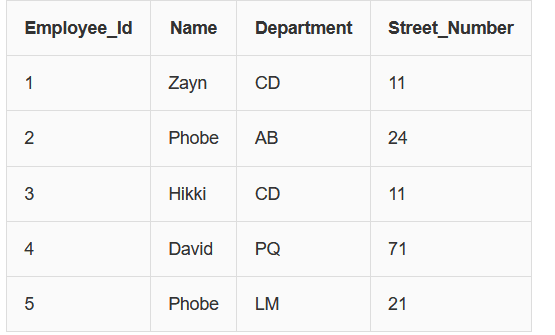
Functional Dependencies:
Employee_Id → Department
Department → Street_Number
From these dependencies we can derive:
Employee_Id → Street_Number
Explanation:
Street_Number depends on Department, and Department depends on Employee_Id.
Therefore Street_Number indirectly depends on Employee_Id.
This is called a Transitive Functional Dependency.
DBMS-এ Functional Dependency
Relational Database Management System (RDBMS)-এ data table আকারে সংরক্ষণ করা হয়।
একটি table বিভিন্ন row এবং column নিয়ে গঠিত।
Column গুলোকে attribute বলা হয় এবং প্রতিটি row একটি record নির্দেশ করে।
DBMS-এ একটি row-কে অনেক সময় tuple বলা হয়।
Example: Employee Table
এখানে দেখা যায় যে Employee_Id জানলে Employee_Name, Employee_Department এবং Salary নির্ধারণ করা যায়।
Functional Dependency কী?
Functional Dependency হলো একটি relation-এর attribute গুলোর মধ্যে relationship।
যদি একটি attribute-এর মান অন্য একটি attribute-এর মান নির্ধারণ করে, তখন তাকে Functional Dependency বলা হয়।
Functional Dependency সাধারণত এভাবে লেখা হয়:
X → Y
অর্থাৎ X attribute দ্বারা Y attribute নির্ধারিত হয়।
Example:
Employee_Id → Employee_Name, Employee_Department, Salary
অর্থাৎ Employee_Id জানলে employee সম্পর্কিত অন্যান্য তথ্য নির্ধারণ করা যায়।
Functional Dependency-এর ধরন
1. Trivial Functional Dependency
যদি dependent attribute determinant-এর subset হয় তাহলে তাকে Trivial Functional Dependency বলা হয়।
Example Table:
| Employee_Id | Name | Age |
|---|---|---|
| 1 | Zayn | 24 |
| 2 | Phobe | 34 |
| 3 | Hikki | 26 |
| 4 | David | 29 |
Example:
{Employee_Id, Name} → Name
এখানে Name ইতিমধ্যে determinant-এর অংশ, তাই এটি Trivial dependency।
2. Non-Trivial Functional Dependency
যদি dependent attribute determinant-এর subset না হয় তাহলে তাকে Non-Trivial Functional Dependency বলা হয়।
Example Table:
| Employee_Id | Name | Age |
|---|---|---|
| 1 | Zayn | 24 |
| 2 | Phobe | 34 |
| 3 | Hikki | 26 |
| 4 | David | 29 |
Example:
Employee_Id → Name
এখানে Name Employee_Id দ্বারা নির্ধারিত হয় এবং Name determinant-এর অংশ নয়।
তাই এটি Non-Trivial Functional Dependency।
3. Multivalued Functional Dependency
যখন একটি attribute একাধিক independent attribute নির্ধারণ করে তখন তাকে Multivalued Functional Dependency বলা হয়।
Example Table:
| Employee_Id | Name | Age |
|---|---|---|
| 1 | Zayn | 24 |
| 2 | Phobe | 34 |
| 3 | Hikki | 26 |
| 4 | David | 29 |
| 4 | Phobe | 24 |
Example:
Employee_Id → {Name, Age}
এখানে Name এবং Age উভয়ই Employee_Id-এর উপর নির্ভরশীল কিন্তু Name → Age বা Age → Name নেই।
তাই এটি Multivalued dependency।
4. Transitive Functional Dependency
যখন একটি attribute অন্য একটি attribute-এর মাধ্যমে পরোক্ষভাবে নির্ভরশীল হয় তখন তাকে Transitive Functional Dependency বলা হয়।
Example Table:
Functional Dependencies:
Employee_Id → Department
Department → Street_Number
তাহলে
Employee_Id → Street_Number
কারণ Street_Number → Department-এর উপর নির্ভরশীল এবং Department → Employee_Id-এর উপর নির্ভরশীল।
এটি একটি Transitive Functional Dependency।
Second Normal Form (2NF) is the second step of database normalization.
The main goal of 2NF is to remove partial dependency from a table.
A table is said to be in Second Normal Form if it satisfies the following conditions:
- The table must already be in First Normal Form (1NF).
- All non-prime attributes must be fully dependent on the entire primary key.
A partial dependency occurs when a non-key attribute depends only on a part of a composite primary key instead of the whole key.
Such dependencies create redundancy and must be removed to achieve 2NF.
Example: Table not in 2NF
Consider the following table EmployeeProjectDetail: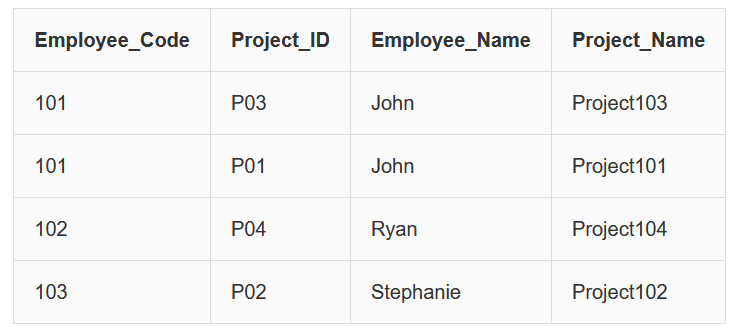
In this table, the primary key is a combination of:
Employee_Code + Project_ID
However we observe the following dependencies:
Employee_Code → Employee_Name
Project_ID → Project_Name
This means:
• Employee_Name depends only on Employee_Code
• Project_Name depends only on Project_ID
Since these attributes depend on only part of the composite key, this creates partial dependency.
Therefore the table is not in Second Normal Form.
Converting the Table into 2NF
To remove partial dependencies, we divide the table into smaller related tables.
EmployeeDetail Table
| Employee_Code | Employee_Name |
|---|---|
| 101 | John |
| 102 | Ryan |
| 103 | Stephanie |
ProjectDetail Table
| Project_ID | Project_Name |
|---|---|
| P03 | Project103 |
| P01 | Project101 |
| P04 | Project104 |
| P02 | Project102 |
EmployeeProject Table
| Employee_Code | Project_ID |
|---|---|
| 101 | P03 |
| 101 | P01 |
| 102 | P04 |
| 103 | P02 |
Now:
• Each table is in 1NF
• All non-key attributes depend on the whole primary key
Therefore the database is now in Second Normal Form (2NF).
Second Normal Form (2NF) হলো database normalization-এর দ্বিতীয় ধাপ।
2NF-এর মূল উদ্দেশ্য হলো table থেকে partial dependency দূর করা।
একটি table তখনই 2NF-এ থাকবে যখন নিচের শর্তগুলো পূরণ হবে:
- Table অবশ্যই First Normal Form (1NF)-এ থাকতে হবে।
- সব non-prime attribute পুরো primary key-এর উপর fully dependent হতে হবে।
Partial Dependency তখন ঘটে যখন কোনো non-key attribute composite primary key-এর একটি অংশের উপর নির্ভরশীল হয়।
Example: 2NF না থাকা Table
এখানে primary key হলো:
Employee_Code + Project_ID
কিন্তু আমরা দেখতে পাই:
Employee_Code → Employee_Name
Project_ID → Project_Name
অর্থাৎ:
• Employee_Name শুধুমাত্র Employee_Code-এর উপর নির্ভরশীল
• Project_Name শুধুমাত্র Project_ID-এর উপর নির্ভরশীল
এটি partial dependency তৈরি করে, তাই table টি 2NF-এ নেই।
Table-কে 2NF-এ রূপান্তর
Partial dependency দূর করার জন্য table-টিকে কয়েকটি ছোট table-এ ভাগ করা হয়।
EmployeeDetail Table
| Employee_Code | Employee_Name |
|---|---|
| 101 | John |
| 102 | Ryan |
| 103 | Stephanie |
ProjectDetail Table
| Project_ID | Project_Name |
|---|---|
| P03 | Project103 |
| P01 | Project101 |
| P04 | Project104 |
| P02 | Project102 |
EmployeeProject Table
| Employee_Code | Project_ID |
|---|---|
| 101 | P03 |
| 101 | P01 |
| 102 | P04 |
| 103 | P02 |
এখন:
• প্রতিটি table 1NF-এ আছে
• সব non-prime attribute পুরো primary key-এর উপর dependent
তাই এখন database টি Second Normal Form (2NF)-এ রয়েছে।
Third Normal Form (3NF)
Third Normal Form (3NF) is the third step of database normalization.
The main goal of 3NF is to remove transitive dependency from a table.
A transitive dependency occurs when a non-key attribute depends on another non-key attribute instead of depending directly on the primary key.
A functional dependency X → Z is called transitive if the following conditions exist:
- X → Y
- Y → Z
- Y does not determine X
This means attribute Z depends on X indirectly through Y.
Rules for Third Normal Form (3NF)
For a table to be in Third Normal Form, it must satisfy the following conditions:
- The table must already be in Second Normal Form (2NF).
- No non-prime attribute should depend transitively on the primary key.
- For every functional dependency X → Z, at least one of the following must hold:
- X is a super key.
- Z is a prime attribute.
If transitive dependency exists, we divide the table into smaller tables so that each non-key attribute depends directly on the primary key.
Example: Table not in 3NF
Consider the following table EmployeeDetail:
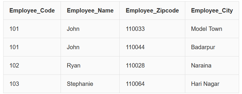
In this table we observe the following functional dependencies:
Employee_Code → Employee_Zipcode
Employee_Zipcode → Employee_City
From these two dependencies we get:
Employee_Code → Employee_City
Here Employee_City depends on Employee_Zipcode, not directly on Employee_Code.
Therefore this is a Transitive Dependency.
Since a non-prime attribute (Employee_City) depends on another non-prime attribute, the table is not in Third Normal Form.
Converting the Table into 3NF
To remove the transitive dependency, we divide the table into two tables.
EmployeeDetail Table
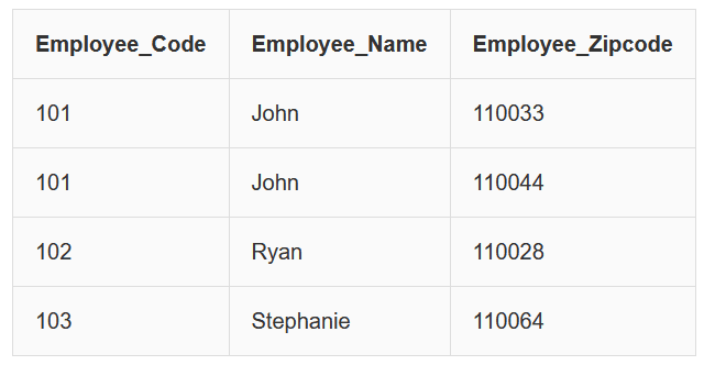
EmployeeLocation Table
| Employee_Zipcode | Employee_City |
|---|---|
| 110033 | Model Town |
| 110044 | Badarpur |
| 110028 | Naraina |
| 110064 | Hari Nagar |
Now:
- Both tables are in Second Normal Form (2NF).
- No transitive dependency exists.
- Each non-key attribute depends directly on the primary key.
Therefore the database is now in Third Normal Form (3NF).
Third Normal Form (3NF)
Third Normal Form (3NF) হলো database normalization-এর তৃতীয় ধাপ।
3NF-এর প্রধান উদ্দেশ্য হলো table থেকে transitive dependency দূর করা।
Transitive Dependency তখন ঘটে যখন একটি non-key attribute অন্য একটি non-key attribute-এর উপর নির্ভরশীল হয় এবং সরাসরি primary key-এর উপর নির্ভরশীল নয়।
একটি functional dependency X → Z তখন transitive হয় যদি:
- X → Y
- Y → Z
- Y → X না হয়
অর্থাৎ Z attribute, X-এর উপর সরাসরি নয় বরং Y-এর মাধ্যমে নির্ভরশীল।
3NF-এর নিয়ম
একটি table তখনই Third Normal Form-এ থাকবে যদি:
- Table অবশ্যই Second Normal Form (2NF)-এ থাকে।
- কোনো non-prime attribute primary key-এর উপর transitively dependent না হয়।
- প্রতিটি functional dependency X → Z এর ক্ষেত্রে নিচের যেকোনো একটি শর্ত সত্য হবে:
- X একটি super key হবে
- Z একটি prime attribute হবে
যদি transitive dependency থাকে তাহলে table-টিকে ছোট ছোট table-এ ভাগ করতে হয়।
Example: 3NF না থাকা Table
এখানে আমরা দেখতে পাই:
Employee_Code → Employee_Zipcode
Employee_Zipcode → Employee_City
তাই,
Employee_Code → Employee_City
এখানে Employee_City সরাসরি Employee_Code-এর উপর নির্ভরশীল নয়, বরং Employee_Zipcode-এর মাধ্যমে নির্ভরশীল।
এটি একটি Transitive Dependency।
তাই table টি 3NF-এ নেই।
Table-কে 3NF-এ রূপান্তর
EmployeeDetail Table
EmployeeLocation Table
| Employee_Zipcode | Employee_City |
|---|---|
| 110033 | Model Town |
| 110044 | Badarpur |
| 110028 | Naraina |
| 110064 | Hari Nagar |
এখন:
- দুটি table-ই 2NF-এ রয়েছে
- কোনো transitive dependency নেই
- সব non-key attribute সরাসরি primary key-এর উপর নির্ভরশীল
তাই database টি এখন Third Normal Form (3NF)-এ রয়েছে।
Database Transaction, ACID Propertise , Deadlock in DBMS
Deadlock in DBMS
A deadlock occurs in a multi-user database environment when two or more transactions wait for each other indefinitely while holding resources required by the others.
In this situation, each transaction holds a resource and waits for another resource that is locked by another transaction. This creates a circular wait condition, and none of the transactions can continue their execution.
Deadlocks prevent the system from progressing and must be resolved by the Database Management System (DBMS).
Example of Deadlock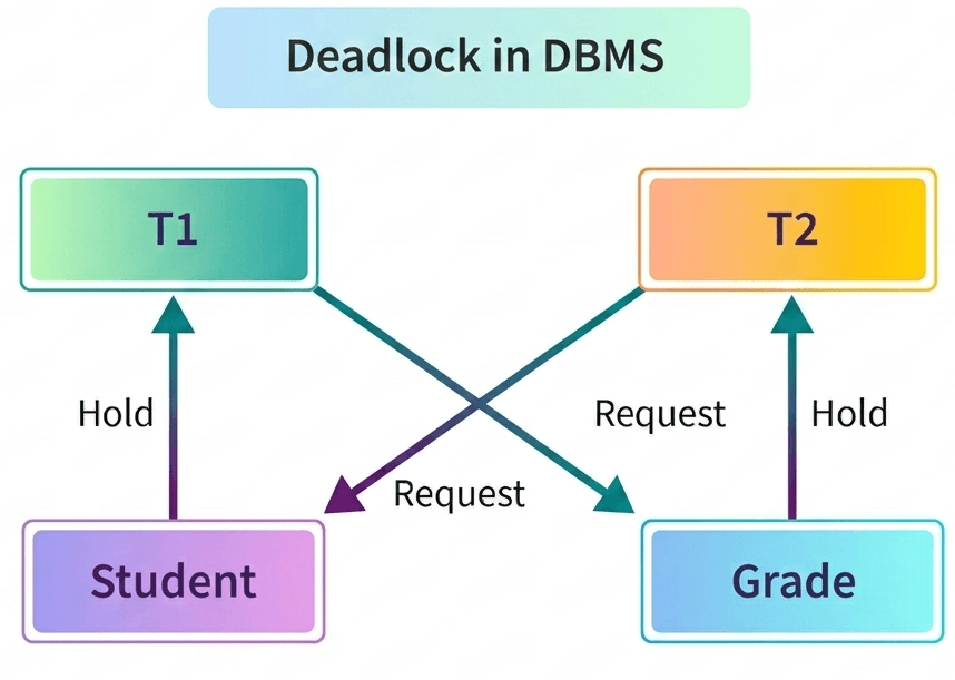
Consider a database that contains two tables: Student and Grade.
| Transaction | Action |
|---|---|
| Transaction 1 | Locks records in the Student table and then tries to update the Grade table. |
| Transaction 2 | Locks records in the Grade table and then tries to update the Student table. |
In this case:
- Transaction 1 holds a lock on the Student table and waits to access the Grade table.
- Transaction 2 holds a lock on the Grade table and waits to access the Student table.
Since both transactions are waiting for each other to release the locked resources, neither of them can proceed. This creates a deadlock situation.
Deadlock Resolution
To resolve a deadlock, the DBMS detects the circular waiting condition and usually aborts one of the transactions.
The aborted transaction releases its locks, allowing the other transaction to continue execution.
DBMS-এ Deadlock
Deadlock হলো এমন একটি অবস্থা যেখানে একাধিক transaction একে অপরের জন্য অপেক্ষা করতে থাকে এবং কেউই তাদের কাজ সম্পন্ন করতে পারে না।
এই পরিস্থিতি ঘটে যখন প্রতিটি transaction একটি resource lock করে রাখে এবং অন্য একটি resource-এর জন্য অপেক্ষা করে যা অন্য transaction দ্বারা lock করা আছে। ফলে একটি circular wait তৈরি হয় এবং system কাজ করতে পারে না।
এই সমস্যা সমাধানের জন্য DBMS হস্তক্ষেপ করে।
Deadlock-এর উদাহরণ
ধরুন একটি database-এ দুটি table আছে: Student এবং Grade।
| Transaction | Action |
|---|---|
| Transaction 1 | Student table-এর কিছু record lock করে এবং পরে Grade table update করার চেষ্টা করে। |
| Transaction 2 | Grade table-এর কিছু record lock করে এবং পরে Student table update করার চেষ্টা করে। |
এখানে দেখা যায়:
- Transaction 1 Student table lock করে রেখেছে এবং Grade table access করার জন্য অপেক্ষা করছে।
- Transaction 2 Grade table lock করে রেখেছে এবং Student table access করার জন্য অপেক্ষা করছে।
ফলে উভয় transaction একে অপরের জন্য অপেক্ষা করছে এবং কোনো transaction এগোতে পারছে না। এই অবস্থাকেই deadlock বলা হয়।
Deadlock সমাধান
Deadlock হলে DBMS circular wait condition সনাক্ত করে এবং সাধারণত একটি transaction abort করে দেয়।
যে transaction abort হয় তার lock release হয়ে যায় এবং অন্য transaction তার কাজ সম্পন্ন করতে পারে।
Deadlock Detection in DBMS
Deadlock detection is a technique used by a Database Management System (DBMS) to identify whether a group of transactions has entered a deadlock state. A deadlock occurs when two or more transactions wait indefinitely for resources that are held by each other.
When a transaction waits too long to obtain a resource such as a lock or CPU resource, the DBMS checks whether the transaction is part of a deadlock situation. To detect this, the system uses a component called a resource scheduler.
The resource scheduler keeps track of:
- Which resources are currently allocated to each transaction.
- Which resources are requested by other transactions.
By analyzing this information, the DBMS can determine whether a deadlock has occurred.
Wait-For Graph Method
One common technique used for deadlock detection is the Wait-For Graph.
In this method:
- Each node in the graph represents a transaction.
- An edge from transaction T1 to T2 means that T1 is waiting for a resource held by T2.
If the wait-for graph contains a cycle (loop), then a deadlock exists.
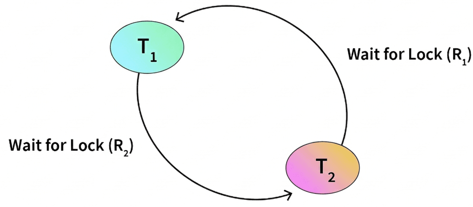
Example
| Transaction | Waiting For |
|---|---|
| T1 | T2 |
| T2 | T1 |
In this situation:
- T1 is waiting for a resource held by T2.
- T2 is waiting for a resource held by T1.
This creates a circular wait, which indicates a deadlock.
The DBMS continuously monitors transactions that are in a waiting state and constructs a wait-for graph. If a cycle is detected, the system identifies the deadlock and resolves it, usually by aborting one of the transactions.
DBMS-এ Deadlock Detection
Deadlock detection হলো এমন একটি পদ্ধতি যেখানে DBMS পরীক্ষা করে দেখে কোনো transaction deadlock অবস্থায় আছে কি না। Deadlock তখন ঘটে যখন একাধিক transaction একে অপরের resource-এর জন্য অনির্দিষ্ট সময় পর্যন্ত অপেক্ষা করে।
যদি কোনো transaction অনেক সময় ধরে resource বা CPU পাওয়ার জন্য অপেক্ষা করে, তখন DBMS পরীক্ষা করে দেখে সেটি deadlock-এর অংশ কি না। এজন্য DBMS একটি resource scheduler ব্যবহার করে।
Resource scheduler নিম্নোক্ত তথ্যগুলো পর্যবেক্ষণ করে:
- কোন transaction কোন resource ব্যবহার করছে।
- কোন transaction অন্য resource-এর জন্য অপেক্ষা করছে।
এই তথ্য বিশ্লেষণ করে DBMS বুঝতে পারে deadlock ঘটেছে কি না।
Wait-For Graph Method
Deadlock detect করার জন্য একটি সাধারণ পদ্ধতি হলো Wait-For Graph।
এই পদ্ধতিতে:
- Graph-এর প্রতিটি node একটি transaction নির্দেশ করে।
- T1 থেকে T2-এর দিকে একটি edge থাকলে বোঝায় T1, T2-এর resource-এর জন্য অপেক্ষা করছে।
যদি graph-এ একটি cycle বা loop তৈরি হয়, তাহলে deadlock রয়েছে।
Example
| Transaction | Waiting For |
|---|---|
| T1 | T2 |
| T2 | T1 |
এখানে:
- T1 অপেক্ষা করছে T2-এর resource-এর জন্য।
- T2 অপেক্ষা করছে T1-এর resource-এর জন্য।
এভাবে একটি circular wait তৈরি হয় এবং deadlock ঘটে।
DBMS অপেক্ষমাণ transaction গুলোকে পর্যবেক্ষণ করে এবং Wait-For Graph তৈরি করে। যদি graph-এ cycle পাওয়া যায়, তাহলে system deadlock শনাক্ত করে এবং সাধারণত একটি transaction abort করে সমস্যাটি সমাধান করে।