Combined Bank
Post: Assistant Programmer ,
Exam Date: 09.06.2023
- User Input = 50
- User Output = 40
- User Inquiries = 35
- User Files = 6
- External Interface = 4
Step 1:
As the complexity adjustment factor is average (given in the question), the scale is set to 3 for each factor.
F = 14 × 3 = 42
Step 2:
Calculate the Complexity Adjustment Factor (CAF) using the formula:
CAF = 0.65 + (0.01 × F)
Substitute F = 42:
CAF = 0.65 + (0.01 × 42) = 1.07
Step 3:
Calculate the Unadjusted Function Points (UFP) using the given values and the corresponding weights (average weighting factors):
UFP = (50 × 4) + (40 × 5) + (35 × 4) + (6 × 10) + (4 × 7)
UFP = 200 + 200 + 140 + 60 + 28 = 628
Step 4:
Calculate the Function Point (FP) using the formula:
FP = UFP × CAF
FP = 628 × 1.07 = 671.96
Final Answer:
The Function Point (FP) is: 671.96
Algorithm to Find the Smallest Element in an Array
START
Step 1 → Initialize an array A with given values.
Step 2 → Create a variable min_value and set it to a large number (e.g., infinity) or the first element of the array.
Step 3 → Loop through each element A[i] in the array starting from the first element.
Step 4 → For each element, check if A[i] is smaller than min_value.
Step 5 → If A[i] < min_value, update min_value to A[i].
Step 6 → Repeat Steps 4 and 5 until all elements have been checked.
Step 7 → Display min_value as the smallest element of the array.
STOP
Given:
- Page reference string: 1, 3, 0, 3, 5, 6, 3
- Number of page frames: 3
Step-by-Step Analysis:
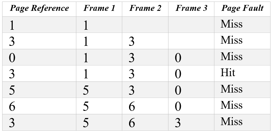
Explanation:
- 1 causes a page fault as it’s not in memory, so it’s loaded into frame 1.
- 3 causes a page fault and is loaded into frame 2.
- 0 causes a page fault and is loaded into frame 3. All three frames are now full.
- 3 is already in memory, so no page fault occurs (Hit).
- 5 causes a page fault and replaces the oldest page in memory, which is 1.
- 6 causes a page fault and replaces the oldest page in memory, which is 3.
- 3 causes a page fault and replaces the oldest page in memory, which is 0.
Total Page Faults:
- 6 Page Faults
Solution:
Step 1: Represent Data and Divisor in Polynomial Form
Data (11100):
x4 + x3 + x2
Divisor (1001):
x3 + 1
Step 2: Append Zeros to the Original Data
Since the divisor is 4 bits, we append 3 zeros to the original data (one less than the number of bits in the divisor). The new data is:
Data after appending zeros: 11100000
Step 3: Perform Binary Division
Now we divide the modified data 11100000 by the divisor 1001.
Division Process:
11111 ← Quotient
—————————–
11100000 ← Dividend (data with zeros)
1001 ← Divisor
———————-
1110000
1001
—————-
111000
1001
—————
11100
1001
————
1110
1001
————
111
Step 4: Determine the Transmitted Value
The remainder 111 is the CRC code. To get the transmitted value, append the remainder to the original data:
Original data: 11100
Remainder: 111
Transmitted Value: 11100111
Impact of Stealing a Private Key in TLS
If an attacker steals the private key of a website that uses Transport Layer Security (TLS) and remains undetected, several serious security threats can occur.
- Decryption of Encrypted Traffic: The attacker can decrypt past and future TLS sessions (if Perfect Forward Secrecy is not used).
- Impersonation: The attacker can impersonate the legitimate website and perform Man-in-the-Middle (MITM) attacks.
- Data Theft: Sensitive data such as usernames, passwords, cookies, and credit card details can be stolen.
- Malware Injection: Malicious content can be injected while appearing as a trusted website.
Mitigation Steps:
- Immediately revoke the compromised certificate.
- Generate a new key pair and install a new certificate.
- Enable Perfect Forward Secrecy (PFS).
- Monitor logs and notify users if required.
TLS-এ Private Key চুরি হলে কী হতে পারে
যদি কোনো attacker একটি TLS ব্যবহারকারী website-এর private key চুরি করে এবং তা ধরা না পড়ে, তাহলে গুরুতর নিরাপত্তা ঝুঁকি তৈরি হয়।
- Encrypted Data Decrypt করা: Perfect Forward Secrecy ব্যবহার না করলে attacker আগের ও ভবিষ্যতের TLS session decrypt করতে পারে।
- Website Impersonation: Attacker আসল website সেজে Man-in-the-Middle (MITM) attack চালাতে পারে।
- Sensitive Data চুরি: Username, password, cookie, credit card তথ্য চুরি হতে পারে।
- Malware Injection: Trusted website-এর মতো দেখিয়ে malicious content ঢুকানো যায়।
সমাধানমূলক ব্যবস্থা:
- Compromised certificate সঙ্গে সঙ্গে revoke করতে হবে।
- নতুন key pair ও certificate তৈরি করতে হবে।
- Perfect Forward Secrecy (PFS) চালু করতে হবে।
- Log monitor করে প্রয়োজনে user-দের জানাতে হবে।
Reasonable Security Policy for Cross-Origin Frame Navigation
Consider two browser frames A and B loaded from different origins. Allowing frame A to navigate frame B to another origin is considered a reasonable security policy only when the display area of A contains part of B and A has control over that area.
Reasons:
- User Awareness: Since frame A visibly contains part of frame B, the user can see the interaction and is less likely to be tricked by hidden or invisible actions.
- UI Control: If A controls the display area of B, it implies an explicit embedding relationship, making navigation intent clearer and more legitimate.
- Clickjacking Prevention: This restriction prevents malicious frames from silently redirecting other frames that are not visually or structurally related.
- Least Privilege Principle: A is granted limited control (navigation only), not full access to B’s content, maintaining origin isolation.
- Maintains Same-Origin Security: While navigation is allowed, reading or modifying B’s data remains restricted, preserving the same-origin policy.
Allowing navigation under these controlled and visible conditions balances usability with security and prevents abuse across origins.
Cross-Origin Frame Navigation-এর জন্য যুক্তিসংগত Security Policy
ধরা যাক browser-এর দুটি frame A এবং B আলাদা origin থেকে load হয়েছে। Frame A কে frame B-কে অন্য origin-এ navigate করতে দেওয়া যুক্তিসংগত হয় শুধুমাত্র তখনই, যখন A-এর display area-এর ভেতরে B-এর একটি অংশ থাকে এবং সেই area-এর উপর A-এর নিয়ন্ত্রণ থাকে।
কারণসমূহ:
- User Awareness: যেহেতু user দৃশ্যমানভাবে frame B-কে frame A-এর মধ্যে দেখতে পায়, তাই গোপনে বা অজান্তে কোনো navigation হওয়ার ঝুঁকি কমে।
- UI Control: A যদি B-এর display area নিয়ন্ত্রণ করে, তাহলে এটি একটি বৈধ embedding সম্পর্ক নির্দেশ করে।
- Clickjacking প্রতিরোধ: এই নিয়ম malicious frame-কে অন্য frame গোপনে redirect করা থেকে বাধা দেয়।
- Least Privilege Principle: A কেবল navigation করতে পারে, B-এর data access করতে পারে না।
- Same-Origin Security বজায় রাখা: Navigation অনুমোদিত হলেও data পড়া বা পরিবর্তন নিষিদ্ধ থাকে।
এই নীতিটি usability ও security-এর মধ্যে ভারসাম্য বজায় রেখে cross-origin অপব্যবহার প্রতিরোধ করে।
Adjacency List vs Adjacency Matrix: When Each is More Efficient
The choice between adjacency list and adjacency matrix depends on the graph’s density and the specific operation being performed. Neither is universally better; each has scenarios where it dominates.
Problems Solved More Efficiently in Adjacency List
Adjacency list stores only the edges that actually exist, making it ideal for sparse graphs where the number of edges is much less than the square of the number of vertices.
- Memory efficiency: Space is O(V + E) instead of O(V²). For a graph with 10,000 nodes and 20,000 edges, the list uses ~30,000 units while the matrix wastes 100,000,000 units.
- Faster traversal of neighbors: To visit all neighbors of a node, the list iterates only through actual edges. The matrix scans an entire row of V entries regardless of how few edges exist.
- Better for DFS and BFS: These algorithms repeatedly ask “what are the neighbors of this node?” The list answers in O(degree) time versus O(V) for the matrix.
- Dynamic graphs: Adding or removing edges is simpler when only existing connections are tracked.
Example: Social networks where most users have hundreds of friends among millions of users. Finding all friends of one user is fast with a list but wasteful with a matrix.
Problems Solved More Effectively in Adjacency Matrix
Adjacency matrix stores a complete V × V table, making it superior for dense graphs and operations that need instant edge existence checks.
- O(1) edge lookup: Checking if an edge exists between two specific nodes takes constant time. In a list, this requires scanning all neighbors of one node, taking O(V) in the worst case.
- Matrix operations: Graph algorithms using linear algebra like Floyd-Warshall (all-pairs shortest path), transitive closure, and eigenvalue computations require the matrix structure.
- Dense graphs: When E is close to V², the matrix uses less overhead than pointer-based lists and benefits from CPU cache locality since data is contiguous.
- Simple implementation: No linked lists or dynamic arrays to manage; a 2D array is straightforward.
Example: A fully connected network topology where every router connects to every other router. Checking direct connectivity between any two routers is instant with a matrix.
Comparison Table:
| Operation | Adjacency List | Adjacency Matrix |
|---|---|---|
| Space (sparse graph) | O(V + E) — efficient | O(V²) — wasteful |
| Space (dense graph) | O(V + E) — similar | O(V²) — acceptable |
| Check edge (u, v) | O(degree) or O(V) | O(1) — instant |
| Find all neighbors | O(degree) — fast | O(V) — must scan row |
| Add/remove edge | O(1) with dynamic list | O(1) |
| Best for | DFS, BFS, sparse graphs | Dense graphs, all-pairs paths |
Key Insight: Use adjacency list when the graph is large and sparse, or when neighbor traversal dominates. Use adjacency matrix when the graph is small and dense, or when edge existence queries and matrix math operations are frequent.
Adjacency List vs Adjacency Matrix: কখন কোনটি বেশি Efficient
Adjacency list এবং adjacency matrix-এর মধ্যে choice graph-এর density এবং perform হওয়া specific operation-এর উপর নির্ভর করে। কোনো একটি universally better নয়; প্রতিটির এমন scenarios আছে যেখানে এটি dominate করে।
Adjacency List-এ বেশি Efficientভাবে Solve হওয়া Problems
Adjacency list শুধু actually exist করা edges store করে, তাই এটি sparse graphs-এর জন্য ideal যেখানে edges-এর সংখ্যা vertices-এর square-এর চেয়ে অনেক কম।
- Memory efficiency: Space O(V + E) O(V²)-এর পরিবর্তে। 10,000 nodes এবং 20,000 edges থাকা graph-এর জন্য list ~30,000 units ব্যবহার করে যখন matrix 100,000,000 units waste করে।
- Faster traversal of neighbors: একটি node-এর সব neighbors visit করতে list শুধু actual edges iterate করে। Matrix V entries-এর পুরো row scan করে কত কম edges থাকুক না কেন।
- DFS এবং BFS-এর জন্য better: এই algorithms বারবার জিজ্ঞেস করে “এই node-এর neighbors কারা?” List O(degree) time-এ উত্তর দেয় matrix-এর O(V)-এর বিপরীতে।
- Dynamic graphs: শুধু existing connections track করলে edges add বা remove করা সহজ।
Example: Social networks যেখানে বেশিরভাগ users-এর millions of users-এর মধ্যে শতাধিক friends থাকে। একজন user-এর সব friends খুঁজতে list দ্রুত কিন্তু matrix wasteful।
Adjacency Matrix-এ বেশি Effectiveভাবে Solve হওয়া Problems
Adjacency matrix একটি complete V × V table store করে, তাই এটি dense graphs-এ এবং instant edge existence checks প্রয়োজন এমন operations-এ superior।<
- O(1) edge lookup: দুটি specific node-এর মধ্যে edge exist করে কিনা check করতে constant time লাগে। List-এর ক্ষেত্রে একটি node-এর সব neighbors scan করতে হয়, worst case-এ O(V)।
- Matrix operations: Floyd-Warshall (all-pairs shortest path), transitive closure, এবং eigenvalue computations এর মতো linear algebra ব্যবহার করা graph algorithms matrix structure প্রয়োজন।
- Dense graphs: E V²-এর কাছাকাছি হলে matrix pointer-based lists-এর চেয়ে কম overhead ব্যবহার করে এবং CPU cache locality-তে benefit পায় কারণ data contiguous।
- Simple implementation: Linked lists বা dynamic arrays manage করার প্রয়োজন নেই; 2D array straightforward।
Example: Fully connected network topology যেখানে প্রতিটি router অন্য প্রতিটি router-এর সাথে connected। যেকোনো দুটি router-এর মধ্যে direct connectivity instant check করা যায় matrix দিয়ে।
Comparison Table:
| Operation | Adjacency List | Adjacency Matrix |
|---|---|---|
| Space (sparse graph) | O(V + E) — efficient | O(V²) — wasteful |
| Space (dense graph) | O(V + E) — similar | O(V²) — acceptable |
| Check edge (u, v) | O(degree) বা O(V) | O(1) — instant |
| Find all neighbors | O(degree) — fast | O(V) — row scan করতে হয় |
| Add/remove edge | Dynamic list-এ O(1) | O(1) |
| Best for | DFS, BFS, sparse graphs | Dense graphs, all-pairs paths |
