Dhaka Wasa, Assistant Maintenance Engineer, 2025

Dhaka WASA

Post: Assistant Maintenance Engineer
Exam Date: 04.7.2025
Exam Taker: BUET

1. Find the Norton equivalent circuit for a DC power supply that has a 30 V terminal voltage when delivering 400 mA, and a 28 V terminal voltage when delivering 600 mA.

Norton Equivalent of the DC Power Supply

Given:

Terminal voltage \(V_1 = 30\,\text{V}\) when delivering \(I_1 = 400\,\text{mA} = 0.4\,\text{A}\)
Terminal voltage \(V_2 = 28\,\text{V}\) when delivering \(I_2 = 600\,\text{mA} = 0.6\,\text{A}\)

Step 1: Find internal resistance
For a practical source (Thevenin form): \(V = V_{th} – I R_{th}\)
So,
\(30 = V_{th} – 0.4R_{th}\)
\(28 = V_{th} – 0.6R_{th}\)
Subtracting equations:
\(30 – 28 = ( -0.4R_{th}) – (-0.6R_{th})\)
\(2 = 0.2R_{th}\Rightarrow R_{th} = 10\,\Omega\)

Step 2: Find \(V_{th}\)
\(30 = V_{th} – 0.4(10)\Rightarrow 30 = V_{th} – 4\Rightarrow V_{th} = 34\,\text{V}\)

Step 3: Convert to Norton
\(R_N = R_{th} = 10\,\Omega\)
\(I_N = \dfrac{V_{th}}{R_{th}} = \dfrac{34}{10} = 3.4\,\text{A}\)

Final Norton Equivalent:

Norton Current: \(I_N = 3.4\,\text{A}\)
Norton Resistance: \(R_N = 10\,\Omega\) (in parallel with the current source)

Equivalent circuit: A 3.4 A current source in parallel with a 10 Ω resistor.

DC Power Supply-এর Norton Equivalent Circuit

প্রদত্ত:

\(I_1 = 0.4\,\text{A}\) হলে terminal voltage \(V_1 = 30\,\text{V}\)
\(I_2 = 0.6\,\text{A}\) হলে terminal voltage \(V_2 = 28\,\text{V}\)

Step 1: Internal resistance বের করা
Practical source-এর জন্য: \(V = V_{th} – IR_{th}\)
তাহলে,
\(30 = V_{th} – 0.4R_{th}\)
\(28 = V_{th} – 0.6R_{th}\)
দুটি সমীকরণ বিয়োগ করলে:
\(2 = 0.2R_{th}\Rightarrow R_{th} = 10\,\Omega\)

Step 2: \(V_{th}\) বের করা
\(30 = V_{th} – 0.4(10)\Rightarrow V_{th} = 34\,\text{V}\)

Step 3: Norton-এ রূপান্তর
\(R_N = R_{th} = 10\,\Omega\)
\(I_N = \dfrac{V_{th}}{R_{th}} = \dfrac{34}{10} = 3.4\,\text{A}\)

চূড়ান্ত Norton Equivalent:

Norton Current: \(I_N = 3.4\,\text{A}\)
Norton Resistance: \(R_N = 10\,\Omega\) (current source-এর সাথে parallel)

Equivalent circuit: একটি 3.4 A current source, যার সাথে parallel-এ একটি 10 Ω resistor থাকবে।

2. Design a three-input XOR gate with the output function X=A⊕B⊕C using 2-input multiplexers.

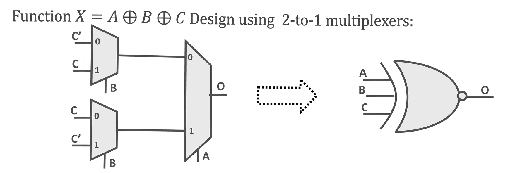
3-input XOR gate using 2:1 muxes: A 3-input XOR gate returns “1” when the odd number of inputs are “1”. The truth table for 3-input XOR gate is shown in figure below.

A	B	C	O
0	0	0	0
0	0	1	1
0	1	0	1
0	1	1	0
1	0	0	1
1	0	1	0
1	1	0	0
1	1	1	1

Truth table for 3-input XOR gate
Let us choose A to be the select of mux closest to output. When A is “0”, output is a function of B and C. So, we need another mux, let us choose B to be the select of this mux. Among the rows with A = 0, when B is “0”, output is equal to C and when B is “1”, output is equal to C’.

Similarly among the rows with A = “1”, when B is “0”, output is equal to C’ and when B is “1”, output is equal to C. The implementation of 3-input XOR gate using 2:1 muxes is shown in figure below.

3. A system uses 16-bit logical address and a page size of 1 KB.
(i) How many pages are in the logical address space?
(ii) How many bits are used for the page number and offset?

The hash function is given as h(k)=k mod 13.
The table size is 13, meaning we have indices from 0 to 12.

Step-by-Step Insertion Process
Key: 10
Hash value: h(10) = 10 mod 13 = 10. Insert 10 at index 10.
Key: 3
Hash value: h(3) = 3 mod 13 = 3. Insert 3 at index 3.
Key: 6
Hash value: h(6) = 6 mod 13 = 6. Insert 6 at index 6.
Key: 16
Hash value: h(16) = 16 mod 13 = 3. Index 3 is occupied. Use linear probing and insert 16 at index 4.
Key: 17
Hash value: h(17) = 17 mod 13 = 4. Index 4 is occupied. Use linear probing and insert 17 at index 5.
Key: 19
Hash value: h(19) = 19 mod 13 = 6. Index 6 is occupied. Use linear probing and insert 19 at index 7.
Final Hash Table

Index	Value
0	–
1	–
2	–
3	3
4	16
5	17
6	6
7	19
8	–
9	–
10	10
11	–
12	–

Summary
The final hash table after inserting all keys using linear probing is as follows:

[ – , – , – , 3 , 16 , 17 , 6 , 19 , – , – , 10 , – , – ]

4. Write a Linux command to count the total number of characters and words from the first 10 lines of a file named wasacustomers.txt.

The hash function is given as h(k)=k mod 13.
The table size is 13, meaning we have indices from 0 to 12.

Index	Value
0	–
1	–
2	–
3	3
4	16
5	17
6	6
7	19
8	–
9	–
10	10
11	–
12	–

Summary
The final hash table after inserting all keys using linear probing is as follows:

[ – , – , – , 3 , 16 , 17 , 6 , 19 , – , – , 10 , – , – ]

5. Given the network 245.248.128.0/20, divide the address space among three departments as follows:
(a) Manager: half of the address space
(b) HR: one-quarter of the address space
(c) Admin: the remaining one-quarter

The hash function is given as h(k)=k mod 13.
The table size is 13, meaning we have indices from 0 to 12.

Index	Value
0	–
1	–
2	–
3	3
4	16
5	17
6	6
7	19
8	–
9	–
10	10
11	–
12	–

Summary
The final hash table after inserting all keys using linear probing is as follows:

[ – , – , – , 3 , 16 , 17 , 6 , 19 , – , – , 10 , – , – ]

6. What will be the output of the following program?
#include int main() {
int i = -1, j = -1, k = 0, l = 2, m;
m = i++ && j++ && k++ || l++;
printf("%d %d %d %d %d", i, j, k, l, m);
return 0;
}

The hash function is given as h(k)=k mod 13.
The table size is 13, meaning we have indices from 0 to 12.

Index	Value
0	–
1	–
2	–
3	3
4	16
5	17
6	6
7	19
8	–
9	–
10	10
11	–
12	–

Summary
The final hash table after inserting all keys using linear probing is as follows:

[ – , – , – , 3 , 16 , 17 , 6 , 19 , – , – , 10 , – , – ]

7. From an Employee table, write SQL statements according to the following question:
(a) Find out the employees who join on the same date.
(b) Find those employees whose salary is greater than 8,000 and less than 25,000.

The hash function is given as h(k)=k mod 13.
The table size is 13, meaning we have indices from 0 to 12.

Index	Value
0	–
1	–
2	–
3	3
4	16
5	17
6	6
7	19
8	–
9	–
10	10
11	–
12	–

Summary
The final hash table after inserting all keys using linear probing is as follows:

[ – , – , – , 3 , 16 , 17 , 6 , 19 , – , – , 10 , – , – ]

Leave a Comment Cancel Reply

You must be logged in to post a comment.

Field Based Job Solution Topic Based QnS IT Job News / Circular

Dhaka WASA Post: Assistant Maintenance Engineer Exam Date: 04.7.2025Exam Taker: BUET

Leave a Comment Cancel Reply

Dhaka WASA

Post: Assistant Maintenance Engineer
Exam Date: 04.7.2025
Exam Taker: BUET